RYS Controlled SAT message passing

The previous posts in this series built a geometric language for David Ng’s Repeat-Your-Self (RYS) construction. In How skip connections define graphs in deep networks I treated a Transformer as a weighted directed graph over residual-stream states; in Similarity of neural networks representations I replaced raw cosine with linear CKA and derived a closed form for the connectome edges; and in Deep Equilibrium Models as a model for RYS I argued that a good RYS window behaves like a quasi-equilibrium operator.

All of that was developed against industrial decoder-only LLMs, exactly the setting of Ng’s original RYS blog post (Ng, 2026), where repeating a block of middle layers of a 27B-parameter model improves MATH and MuSR without changing a single weight. That is a striking phenomenon, but it is an awkward laboratory: the model is enormous, the benchmarks are noisy, the data is uncontrolled, and every ablation costs a GPU afternoon.

This post reports the opposite move. I build a small, fully controlled testbed where I know the ground truth exactly, I can sweep depth and out-of-distribution difficulty at will, and a full RYS intervention map costs minutes on a laptop. The goal is not to beat a benchmark. It is to turn the RYS story into a predictive theory of when and where repeating a block helps, grounded in the geometry of intermediate representations, and then to test that theory’s quantitative predictions.

The headline is that RYS keeps working at small scale, and that its benefit is predictable from two scalar summaries of the residual stream — a magnitude \(\rho\) and a phase \(\phi\) — exactly as the closed-form CKA decomposition suggests.

Why a controlled task at all

Two motivations, one scientific and one practical.

Reusable computation as a first-class object. RYS is an instance of a much older idea: decouple the amount of computation a network performs from the number of parameters it stores. Weight-tied recurrence (Universal Transformers (Dehghani et al., 2019)), implicit fixed-point models (Deep Equilibrium Models (Bai et al., 2019)), and the recent recursive-reasoning models HRM/TRM and GRAM (Baek et al., 2026) all share this premise: a compact set of shared transition functions, applied many times, can implement deep reasoning. RYS is the post-hoc version of the same premise — it asks whether a block that a network already learned as a feed-forward stack can be re-traversed to buy extra computation for free. If yes, we are trading FLOPs for parameters after training, which is precisely the lever that matters when memory, not compute, is the binding constraint.

A clear, verifiable problem. To study this we want a task where (i) the ground truth is exact, (ii) difficulty is a tunable knob, and (iii) success is checkable, not approximate. Boolean satisfiability is the natural choice.

The problem: 3-SAT assignment generation

A 3-SAT instance is a Boolean formula in conjunctive normal form where every clause has exactly three literals:

\[\Phi(x_1,\dots,x_n) \;=\; \bigwedge_{c=1}^{m} \big(\ell_{c,1} \vee \ell_{c,2} \vee \ell_{c,3}\big), \qquad \ell_{c,s} \in \{x_k,\, \neg x_k\}.\]

A clause is satisfied if at least one of its literals is true; the formula is satisfied if all clauses are. An assignment is a vector \(a \in \{0,1\}^n\). The decision problem “is \(\Phi\) satisfiable?” is the canonical NP-complete problem; the search problem “produce a satisfying \(a\)” is what we ask the network to do.

Concretely, the dataset is generated as follows (everything is deterministic given a seed, so runs are reproducible):

Sample a planted assignment \(a^\star \in \{0,1\}^n\) uniformly.
Sample \(m\) clauses, each guaranteed to be satisfied by \(a^\star\) (so the formula is satisfiable by construction).
Compute the brute-force satisfying set for \(n \le 20\) variables to confirm satisfiability and to expose the full solution structure.

The in-distribution split uses \(n=6\) variables and \(m=24\) clauses; the out-of-distribution (OOD) split uses larger formulas, \(n=8\), \(m=34\), a scale the network never sees in training. Test and OOD are deliberately different: test measures generalisation to fresh formulas of the same size, while OOD measures whether the network learned an algorithm that transfers to larger, harder instances. The gap between them is the central quantity for any claim about reusable computation.

The verifier and the right metric

An early mistake (worth recording) was to supervise the model to reproduce the lexicographically first brute-force assignment and to score exact match against it. That is scientifically wrong: most satisfiable 3-SAT formulas have many valid assignments, and punishing the model for finding a different valid solution conflates “wrong” with “non-canonical”. A deterministic model that must average over many valid targets is actively pushed toward an invalid midpoint.

The fix is a verifier-based objective. Let \(p_k = \sigma(\text{logit}_k)\) be the predicted probability that \(x_k = 1\). The differentiable soft-SAT loss is the mean negative log-probability that each clause is satisfied, treating literals as independent:

\[\mathcal{L}_{\text{SAT}} = -\frac{1}{m}\sum_{c=1}^{m} \log\!\Big(1 - \prod_{s=1}^{3}\big(1 - q_{c,s}\big)\Big), \qquad q_{c,s} = \begin{cases} p_{k(c,s)} & \text{if } \ell_{c,s}=x_{k},\\ 1 - p_{k(c,s)} & \text{if } \ell_{c,s}=\neg x_{k}. \end{cases}\]

The primary metric is the valid-assignment rate: the fraction of formulas for which the hard prediction \(a_k = \mathbb{1}[p_k > \tfrac12]\) satisfies every clause, checked by an exact verifier. Exact match to the canonical assignment is kept only as a diagnostic. This is the same philosophy GRAM uses for N-Queens and Graph Coloring (Baek et al., 2026): score constraint satisfaction, not identity to one arbitrary solution.

Architectures, and the lesson they taught

I went through three architectures, and the failures were as informative as the successes.

Flat token Transformer. Serialise the CNF as tokens, read a SAT/UNSAT bit from a [CLS] position. This learns the decision task weakly (≈ 0.63 accuracy at the threshold) and, tellingly, its CKA connectome is a single high-similarity plateau from layer ~5 onward: after the formula is compressed into a bit, the late layers barely move the representation. There is no encoder→reasoning→decoder tripartition because the task exerts no pressure to maintain a rich late-layer representation. RYS on such a model produces only tiny, position-dependent effects (a fraction of a percent), exactly because most windows sit in a near-identity plateau.

Factorised CNF Transformer with variable-query tokens. Move to assignment generation and append one query token \(x_k\text{?}\) per variable, forcing the final layers to prepare a structured per-variable logit. This raises validity to ≈ 0.28 in-distribution but stays far too low for a clean RYS study, and adding depth (8 → 16 layers) does not help. The model is still being asked to discover the clause-variable graph from scratch.

Clause-variable message passing. Give the network the structure that SAT actually has. The formula is a bipartite graph: variable nodes on one side, clause nodes on the other, with a signed edge whenever a variable appears in a clause. One round of message passing is

\[\underbrace{m_c = \textstyle\sum_{v \in c}\phi(h_v, s_{c,v})}_{\text{variables}\to\text{clauses}}, \quad \underbrace{m_v = \textstyle\sum_{c \ni v}\psi(h_c, s_{c,v})}_{\text{clauses}\to\text{variables}},\]

with residual updates on both node types. This is the NeuroSAT recipe (Selsam et al., 2019). It nearly doubles in-distribution validity (≈ 0.52) and roughly quintuples OOD validity relative to the flat model, and — crucially — it gives RYS a clean meaning: each round is one iteration of a shared-structure update, so repeating a window of rounds is literally “reason for more steps”.

The architectural lesson is blunt: do not ask a generic model to rediscover a structure you already know. Give it the bipartite graph and the residual-stream geometry becomes interpretable.

From rounds to an iterated operator

Write the variable residual stream after round \(t\) as \(x_t\). With a pre-norm round (LayerNorm inside the update, residual addition left clean),

\[x_{t+1} = x_t + F_t(x_t),\]

so the recursion telescopes exactly:

\[x_j = x_i + \mathbf{S}_{i,j}, \qquad \mathbf{S}_{i,j} = \sum_{k=i}^{j-1} F_k(x_k).\]

This is the same object as in the LLM posts, now realised in a tiny solver we fully control. If we additionally tie the round weights, \(F_t \equiv F\), the stack becomes a genuine iterated map \(x_{t+1} = x_t + F(x_t)\) whose repeated application approaches a fixed point \(x^\star = x^\star + F(x^\star)\), i.e. \(F(x^\star)=0\). That is precisely the Deep Equilibrium reading (Bai et al., 2019): the saturation of accuracy with more rounds is the network reaching its equilibrium, and RYS is one extra Newton-like step on the same operator.

The rho/phi decomposition and the closed-form CKA

Define two scalar summaries of the segment \([i,j)\) of the residual stream — a relative magnitude and an alignment phase:

\[\rho_{i,j} = \frac{\lVert \mathbf{S}_{i,j}\rVert_F}{\lVert x_i\rVert_F}, \qquad \cos\phi_{i,j} = \frac{\langle x_i,\, \mathbf{S}_{i,j}\rangle_F}{\lVert x_i\rVert_F\,\lVert \mathbf{S}_{i,j}\rVert_F}.\]

Substituting \(x_j = x_i + \mathbf{S}_{i,j}\) into the cosine similarity gives the closed form derived in the earlier post:

\[C_{ij} = \frac{1 + \rho_{i,j}\cos\phi_{i,j}}{\sqrt{1 + \rho_{i,j}^{2} + 2\rho_{i,j}\cos\phi_{i,j}}}.\]

Two regimes follow immediately. In the plateau / small-force regime \(\rho \to 0\),

\[1 - C_{ij} \approx \tfrac{1}{2}\,\rho_{i,j}^{2}\,\sin^{2}\phi_{i,j} + \mathcal{O}(\rho^{3}),\]

so high CKA simply means the block is letting the identity edge carry the representation. In the active / large-force regime \(\rho \gtrsim 1\), the similarity drops toward \(\cos\phi\) and the late state forgets \(x_i\).

What RYS does to rho, phi, and CKA

RYS duplicates the block, injecting a second copy of the cumulative residual on a displaced trajectory. Linearising each \(F_k\) around the first-pass state shows that, to leading order,

\[\boxed{\;\rho_{i,j}^{\text{RYS}} \approx 2\,\rho_{i,j}, \qquad \cos\phi_{i,j}^{\text{RYS}} \approx \cos\phi_{i,j}.\;}\]

The magnitude doubles, the phase is preserved. Plugging the doubled force into the plateau expansion gives a sharp, falsifiable prediction:

\[1 - C_{ij}^{\text{RYS}} \approx 4\,\bigl(1 - C_{ij}\bigr) + \mathcal{O}(\rho^{3}).\]

The plateau is broken precisely inside the duplicated window, and nowhere else. Outside the block, the connectome is unchanged. This is the quantitative content of “RYS densifies only the central reasoning sub-DAG”.

Three dynamical-systems diagnostics

The DEQ post listed three conditions a useful RYS window should satisfy. The controlled solver lets us measure all three:

Residual-field stationarity. The second traversal should reapply a similar update, not invent a new one: \(\lVert \mathbf{S}^{(1)}_{i,j}\rVert / \lVert \mathbf{S}^{(0)}_{i,j}\rVert \approx 1\) with high alignment. Empirically this shows up as the doubling \(\lVert \mathbf{S}^{\text{RYS}}\rVert / \lVert \mathbf{S}^{(0)}\rVert \approx 2\) and a near-zero phase shift.
Junction mismatch. The loop feeds \(x_j\) back into the layer that was trained to consume \(x_i\). Safe windows keep \(x_j\) on the input manifold of layer \(i\); we measure the standardised distance between the two activation clouds.
Block-Jacobian stability. With \(T_{i:j}(x) = x + \mathbf{S}_{i,j}(x)\), the dominant singular value of \(\partial T_{i:j}/\partial x\) should be near 1 — large enough to refine, not so large as to send the decoder an alien state. We estimate it by power iteration using forward- and reverse-mode autodiff, so no dense Jacobian is ever formed.

The strong hypothesis is that windows with positive \(\Delta\) validity are exactly those with the stationary, low-mismatch, marginally-stable signature.

The experiments

Every cycle below is logged with parameters, seeds, and saved artifacts in the project’s research diary; the numbers here are from the saved summary.json files.

Binary SAT classification (the plateau, and why it is a poor laboratory)

A factorised CNF classifier trained on balanced 4-var / 12-clause 3-SAT reaches ≈ 0.79 validation accuracy. Its 32-layer CKA connectome is a near-plateau from layer ~8 on (mean CKA ≈ 0.99 in the late band vs ≈ 0.58 early). A full strict upper-triangular RYS \(\Delta\)-accuracy map (496 windows per split) shows the predicted pattern — early duplication hurts, broad late windows help — but the effect is tiny (best \(\Delta \approx +0.3\) to \(+1.0\) percentage points) and test- and OOD-optimal windows disagree. This is the regime where RYS can only do a little, because most of the network is in representational stasis. Useful as a control; not the place to test a theory.

Message-passing solver and the validity-vs-rounds curve

The clause-variable solver trained with the verifier objective and deep supervision gives, across depths 8 / 16 / 32 rounds:

rounds	val valid	test valid	OOD valid
8	0.522	0.532	0.377
16	0.521	0.525	0.409
32	0.521	0.535	0.400

The validity-vs-rounds curve — reading out the assignment after each round — is the cleanest evidence for the iterated-operator picture. In-distribution it rises steeply and saturates by round ~7; OOD it keeps climbing with more rounds (L32 reaches its OOD peak around round 27). Useful reasoning depth scales with problem hardness, which is exactly why RYS — adding reasoning iterations to a trained model — should help most OOD. The RYS \(\Delta\)-validity maps confirm the prediction: the best windows are early-to-middle rounds (the steep part of the curve), the effect grows with depth (best \(\Delta\) validity +0.024 → +0.039 → +0.055 from L8 to L32), and it is selective rather than uniform.

Cycle 6: testing the rho/phi predictions directly

The final cycle makes the residual stream additive (pre-norm), so the \(\rho/\phi\) decomposition is exact, and runs the full validation pipeline on a 16-round solver: measure \(\rho_{i,j}\) and \(\cos\phi_{i,j}\) from the raw variable stream, test the plateau prediction against the measured CKA, then for the best \(\Delta\)-validity windows test the doubling law and the three dynamical diagnostics.

The 16-round pre-norm solver reaches baseline validity 0.547 / 0.513 / 0.384 on val / test / OOD. Three predictions are tested.

(a) The plateau formula predicts the ordering of the connectome almost perfectly, but not its scale. Across all 120 layer pairs, the Spearman correlation between the predicted \(\tfrac12\rho^2\sin^2\phi\) and the measured \(1-\mathrm{CKA}\) is 0.991. The Pearson correlation is only 0.66, and the scatter below shows why: this solver operates at \(\rho \approx 1\) (median relative force 1.03, median \(\cos\phi \approx 0.73\)), i.e. the active regime, not the deep small-force plateau of a 27B LLM. The quadratic small-force expansion therefore overshoots the magnitude badly, while the cross-term \(\mathcal{Q}^2\) — which the decomposition flags as the leading term once the residual is incoherent with the identity stream — is the better magnitude predictor (Pearson 0.90, Spearman 0.96). The rank structure of the connectome is exactly what the geometry says it should be; the absolute scale needs the full closed form, not the leading term.

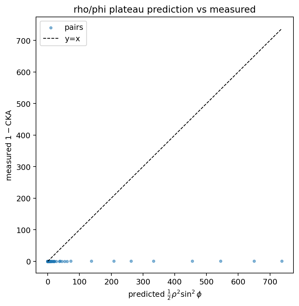
rho phi plateau prediction vs measured — **Plateau prediction vs measured.** Each point is a layer pair. The small-force prediction (x) is rank-faithful (Spearman 0.99) but overshoots in magnitude because the SAT solver lives at \(\rho\approx 1\), off the plateau where the leading quadratic term is valid.

(b) RYS quadruples \(1-\mathrm{CKA}\) inside the duplicated window. For the best windows, the in-window mean ratio \((1-\mathrm{CKA}^{\text{RYS}})/(1-\mathrm{CKA})\) clusters around the predicted 4: 4.03 for window \((13,15)\), 4.19 for \((11,15)\), 4.49 for \((12,15)\), drifting higher (5–6.5) for the tightest windows as higher-order terms enter at \(\rho\approx 1\). The residual-force ratio is \(\approx 1.6\) (predicted 2; below 2 precisely because the second pass runs on a displaced trajectory at non-small \(\rho\)), and the phase is approximately preserved (\(\Delta\cos\phi \approx -0.04\)). Direction and the headline factor of four are confirmed.

(c) The windows that help carry the predicted dynamical signature. The OOD \(\Delta\)-validity map is negative for every early-start window and positive only for a compact late block (start rounds 11–13, end 13–15):

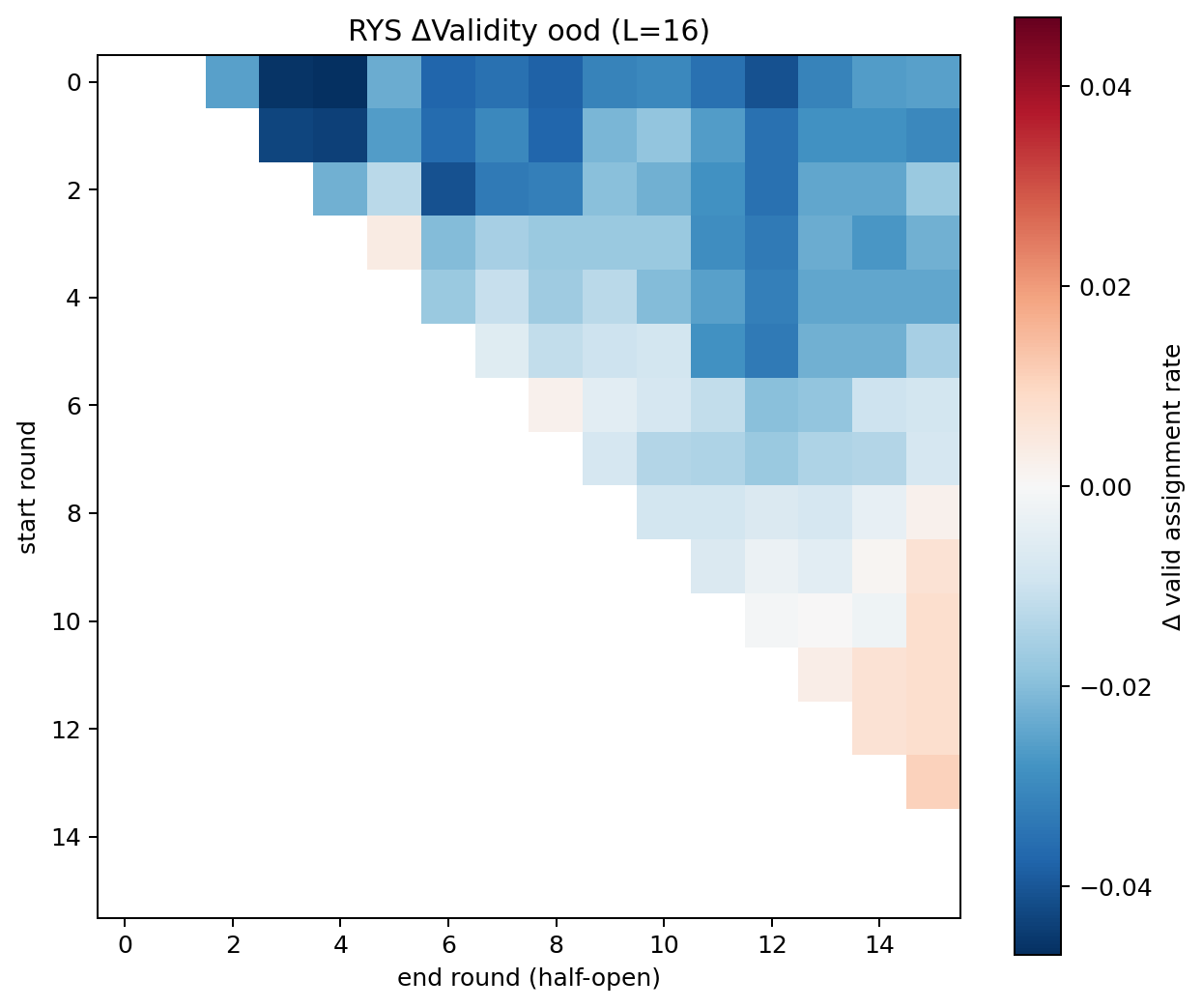
RYS Delta validity OOD heatmap — **RYS \(\Delta\) validity (OOD).** Repeating early rounds is harmful (blue); the only beneficial windows (red) are the late reasoning block — exactly the windows with the cleanest x4 amplification, lowest junction mismatch, and smallest Jacobian.

Linking the diagnostics window-by-window:

window	\(\Delta\) valid (OOD)	\(1-\mathrm{CKA}\) ratio	junction mismatch	Jacobian \(\sigma_{\max}\)
(13, 15)	+0.0107	4.03	0.17	2.07
(12, 15)	+0.0078	4.49	0.20	2.73
(11, 15)	+0.0078	4.19	0.30	3.42
(12, 14)	+0.0068	5.23	0.18	2.70
(11, 14)	+0.0068	5.52	0.27	3.09

The single best OOD window \((13,15)\) also has the lowest junction mismatch (0.17) and the smallest block-Jacobian spectral radius (2.07) — the most stable, most on-manifold loop. This is the strong hypothesis in action: among late high-CKA windows, the one whose repeated map is most stable and least distribution-shifting is the one that helps most out of distribution.

The validity-vs-rounds curve from the depth sweep makes the iterated-operator reading concrete: in-distribution accuracy saturates quickly, while the harder OOD instances keep improving with depth, which is why adding reasoning iterations (RYS) on a late stable block helps most precisely on OOD.

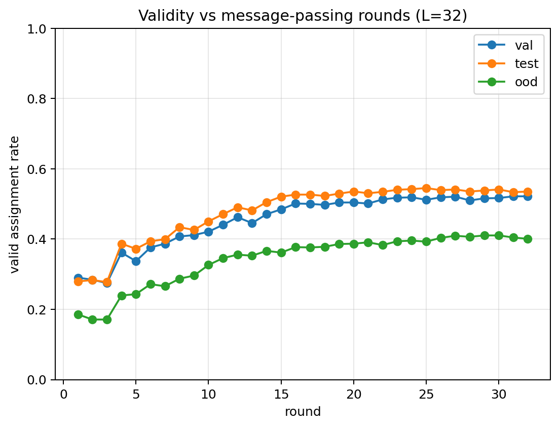
validity vs message-passing rounds — **Validity vs message-passing rounds (32-round solver).** Reading the assignment out after each round: in-distribution saturates early (fixed point), OOD keeps climbing — useful reasoning depth scales with problem hardness.

What this buys us

Three claims, increasingly strong.

RYS is not an artifact of scale. It reproduces in a sub-megabyte solver on a task with exact ground truth. Whatever RYS is, it is not a quirk of 27B-scale pre-training.
The benefit is predictable from geometry. The \(\rho/\phi\) decomposition ties the empirical CKA connectome to the structural recursion, and the doubling law turns “which window helps?” into a measurement on the base model, before any behavioural sweep.
RYS is a controlled exchange of compute for parameters. Reusing a stable, stationary block is one more step of an equilibrium operator. This is the same lever as Universal Transformers, DEQs, and recursive-reasoning models (Dehghani et al., 2019; Bai et al., 2019; Baek et al., 2026), but applied after training, with no new weights.

Relation to recursive-reasoning models

The recent Generative Recursive Reasoning framework (Baek et al., 2026) formalises the family this work lives in: recursive models that refine a latent state with shared transitions, decouple depth from parameters, use deep supervision, scale at inference by depth, and are evaluated on multi-solution constraint problems by constraint validity. Our message-passing solver is an independent reconstruction of that setup, and RYS is its depth-based inference scaling applied post hoc. Where GRAM goes further — and where this testbed should go next — is stochasticity: a deterministic solver on a multi-solution problem mode-collapses, which likely caps our validity near 0.52. Adding stochastic latent transitions and scoring coverage (distinct valid solutions over many samples) is the natural next experiment. Our distinctive angle remains the predictive side: using the CKA magnitude/phase geometry to forecast which windows are safe to repeat, rather than only measuring that repetition helps.

Cycle 7: stochastic transitions, depth and width

A deterministic solver has a structural problem on a multi-solution task. Most satisfiable 3-SAT formulas admit many satisfying assignments, so during training different formulas pull the same variable in opposite directions and the model learns to average. But the average of two valid assignments is usually invalid:

\[\tfrac{1}{2}\big((1,0,0) + (0,1,1)\big) = (0.5,\,0.5,\,0.5) \;\xrightarrow{\text{round}}\; (0,0,0),\]

which can falsify a clause that both endpoints satisfied. This mode collapse is the most likely reason validity plateaus near 0.52 regardless of depth.

The fix, following GRAM (Baek et al., 2026), is to make each round a stochastic transition. Where the deterministic round is

\[x_{t+1} = x_t + F(x_t),\]

the stochastic round adds a learned Gaussian guidance to the deterministic update \(u_t = F(x_t)\):

\[x_{t+1} = x_t + u_t + \varepsilon_t, \qquad \varepsilon_t \sim \mathcal{N}\!\big(\mu_\theta(u_t),\, \sigma_\theta^2(u_t)\,I\big),\]

realised with the reparameterisation trick so it stays differentiable:

\[\varepsilon_t = \mu_\theta(u_t) + \sigma_\theta(u_t)\odot \eta, \qquad \eta \sim \mathcal{N}(0, I).\]

The mean \(\mu_\theta\) is a learned drift — where to steer the reasoning — and \(\sigma_\theta\) is learned exploration — how much a given state may vary. Running the model \(N\) times on the same formula now traces \(N\) different reasoning paths, each able to commit to a different valid assignment instead of collapsing to an invalid midpoint.

Training. We keep the verifier-based soft-SAT loss (it rewards any valid assignment, so distinct samples are all “correct”) and add a small penalty that keeps \(\sigma\) from collapsing to zero — otherwise the optimiser would simply turn the noise off and recover the deterministic model. The clean probabilistic version is an ELBO over latent trajectories (Baek et al., 2026); we start with the lighter sampled objective plus a variance floor.

Inference: depth and width. The verifier makes two new metrics cheap:

\[\text{valid@}N = \mathbb{1}\Big[\exists\, i \le N:\ a^{(i)} \text{ satisfies } \Phi\Big], \qquad \text{coverage} = \frac{\#\{\text{distinct valid } a^{(i)}\}}{\#\{\text{valid } a^{(i)}\}}.\]

valid@N measures whether sampling \(N\) paths finds a solution (almost free, and usually far above single-sample validity); coverage measures whether the paths are genuinely diverse or collapse to one mode.

The link to RYS. Depth and width become two complementary axes of test-time compute, exactly as in GRAM:

Depth (RYS): repeat a window of rounds — reason longer along one path.
Width (stochasticity): sample more paths in parallel.

This raises sharp, testable questions that the deterministic model could not even pose: does RYS help single-sample validity or coverage more? Does a window with a stable block Jacobian (small \(\sigma_{\max}\), as Cycle 6 measured) produce more reliable stochastic trajectories? And does the \(\rho/\phi\) decomposition still describe the deterministic part \(F\) once a stochastic component rides on top of it? The RYS surgery and the CKA/\(\rho/\phi\) analysis are applied to the deterministic operator \(F + \mu_\theta\); the noise is the extra width axis layered on the same geometry.

First result: a negative one, honestly reported. With a light variance floor (target std 0.1, penalty weight \(10^{-2}\)) the stochastic solver matches the deterministic one on single-sample validity (val 0.512 vs 0.514, test 0.540 vs 0.525, OOD 0.363 vs 0.379) but the width axis barely moves:

split	det. single	stoch. single	stoch. valid@20	stoch. coverage
val	0.514	0.512	0.533	0.55
test	0.525	0.540	0.567	0.59
OOD	0.379	0.363	0.387	0.41

valid@20 sits only ~2–3 points above single-sample, and coverage is below 1, meaning the twenty sampled trajectories almost always collapse to the same assignment. The optimiser drove \(\sigma\) down to the floor and effectively recovered the deterministic model — exactly the failure mode the variance floor was meant to prevent, just with too weak a floor. RYS on the late window adds its usual small positive nudge on top, independent of sampling.

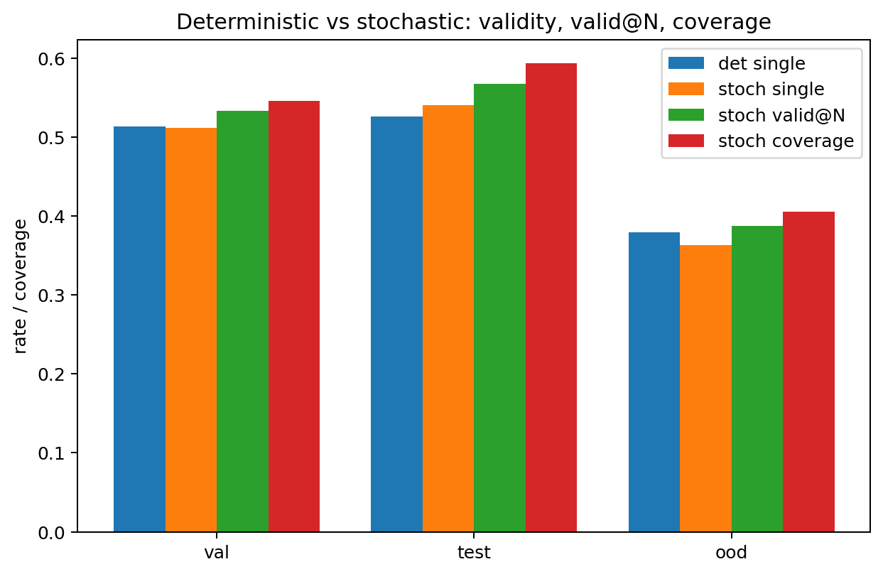
deterministic vs stochastic validity, valid@N, coverage — **Deterministic vs stochastic.** With a weak variance floor the sampled trajectories collapse (coverage < 1), so valid@20 barely exceeds single-sample validity. Breaking the ceiling needs stronger exploration pressure.

The lesson matches GRAM’s own finding that naive noise is not enough: meaningful multi-trajectory behaviour needs either a much stronger exploration incentive or the principled ELBO with a target-conditioned posterior (Baek et al., 2026). The mechanism, metrics, and depth/width harness are now in place; the next iteration is to crank the variance floor (and/or add an entropy/coverage reward) and, if that is still insufficient, move to the amortised-variational objective. This is the cleanest open thread of the programme: we have shown where the deterministic ceiling comes from and built the apparatus to break it, but a light Gaussian guidance alone does not.

Open directions and other datasets

The harness is deliberately dataset-agnostic; the verifier objective only needs a clause tensor. Natural extensions:

Depth-controlled Horn-SAT / unit propagation, where the number of propagation steps to a conflict is a known knob — the cleanest test of “useful depth scales with hardness”.
2-SAT implication-graph reachability, a pure message-passing target with controllable chain length for OOD.
Graph coloring and N-Queens, to connect directly to the GRAM benchmarks and to coverage metrics (Baek et al., 2026).
Stochastic transitions + coverage, to break the deterministic mode-collapse ceiling.
Weight-tied rounds, to make the DEQ fixed-point reading literal and to test whether RYS approximates a Newton step on \(F\).

Reproducibility

Everything is in the rys project. The core pieces are rys.sat_data (generator, verifier, soft-SAT loss), rys.sat_message_passing (the pre-norm / weight-tied clause-variable solver), rys.residual_force and rys.theory_validation (the \(\rho/\phi\) decomposition and diagnostics), and rys.surgery.apply_rys (the no-weight RYS replay). The message-passing depth sweep and the theory-validation pipeline are scripts/run_sat_messagepassing_experiment.py and scripts/run_sat_theory_validation.py. A representative command:

python scripts/run_sat_theory_validation.py --depth 16 --seed 44

All splits are deterministic given the seed, labels are exact by brute force, and the RYS convention is the half-open window of apply_rys (duplicated rounds start..end-1, n_repeats=2), matching the closed-form prediction in predict_cka_under_rys.

References

Ng, D. N. (2026). LLM Neuroanatomy: How I Topped the LLM Leaderboard Without Changing a Single Weight. https://dnhkng.github.io/posts/rys/
Dehghani, M., Gouws, S., Vinyals, O., Uszkoreit, J., & Kaiser, L. (2019). Universal Transformers. International Conference on Learning Representations.
Bai, S., Kolter, J. Z., & Koltun, V. (2019). Deep Equilibrium Models. Advances in Neural Information Processing Systems.
Baek, J., Jo, M., Kim, M., Ren, M., Bengio, Y., & Ahn, S. (2026). Generative Recursive Reasoning. ArXiv Preprint ArXiv:2605.19376.
Selsam, D., Lamm, M., Bünz, B., Liang, P., de Moura, L., & Dill, D. L. (2019). Learning a SAT Solver from Single-Bit Supervision. International Conference on Learning Representations.

A controlled testbed for Repeat-Your-Self — SAT solving, message passing, and a predictive rho/phi theory

RYS Controlled SAT message passing

Why a controlled task at all