Similarity of neural networks representations

In yesterday’s post on How skip connections define graphs in deep networks I built an \(L\times L\) functional connectome of a Transformer by taking pairwise cosine similarities of layer activations. That edge had a clean closed form in the cumulative residual force \(\rho_{i,j}\) and the residual-vs-identity angle \(\phi_{i,j}\), and the same closed form predicted that David Ng’s Repeat Your Self (RYS) construction (Ng, 2026) amplifies the off-plateau deviation in the central reasoning block by a factor of four.

The cosine connectome is almost the right object. Its three weaknesses are that (i) it depends on the basis chosen for the residual stream, so two layers that differ only by a permutation of channel indices are not assigned similarity 1; (ii) it inherits a layer-depth offset from the un-centered mean of activations that contaminates every entry of the matrix; and (iii) it cannot meaningfully compare layers of different widths. The right replacement is linear Centered Kernel Alignment (CKA), the cosine of the similarity-of-similarities matrix that sits one tensor level above the residual stream (Kornblith et al., 2019). This post derives the CKA edge inside the residual recursion of yesterday’s post, validates the resulting plateau formula on synthetic and real Qwen3.6-27B activations, and uses it to interpret David Ng’s RYS-on-MATH intervention map. The empirical pay-off is that the central plateau of the CKA matrix on GSM8K and MMLU-Philosophy hosts the windows whose RYS duplication actually moves the needle on math benchmarks — turning the correlational similarity index into a defensible prior for which RYS surgeries to attempt.

Why linear CKA is the right edge

Three desiderata pin down the choice of similarity index for layer-to-layer comparisons in modern Transformers.

Invariance to orthogonal transformation of the feature axes. Gradient descent inherits a rotational symmetry of the input basis under any orthogonal \(U\) via \(X \mapsto XU\), \(W \mapsto U^TW\), including the special case where \(U\) is a permutation matrix. We want the similarity to assign 1 to representations that differ only by such a rotation.
Invariance to global isotropic scaling: \(X \mapsto \alpha X\) should not change the similarity, for any \(\alpha > 0\).
Non-invariance to arbitrary invertible linear transformation. A theorem of (Kornblith et al., 2019) (their 2.1) shows that any similarity index invariant to invertible linear transformations becomes mathematically constant in the high-width regime \(d \geq N\). Since modern LLMs evaluate hidden states of width \(d \in [4096, 16384]\) on \(N \sim 10^3{-}10^5\) tokens, this regime is exactly the one we care about, and CCA-class indices (CCA, SVCCA, PWCCA, linear regression \(R^2\)) all collapse to the same number for every full-rank input.

Linear CKA satisfies (1) and (2) without falling into the trap (3). Its formula on centered activation matrices \(\tilde X = HX\) with \(H = I_n - \tfrac{1}{n}\mathbf 1 \mathbf 1^T\) is

\[\mathrm{CKA}(\tilde X, \tilde Y) = \frac{\|\tilde Y^T \tilde X\|_F^2}{\|\tilde X^T \tilde X\|_F\,\|\tilde Y^T \tilde Y\|_F}. \tag{1}\label{eq:linear-cka}\]

The single observation that does all the work in the rest of this post is the geometric reading of \eqref{eq:linear-cka}: linear CKA is the cosine of the angle between the vectorised centered Gram matrices of the two representations,

\[\mathrm{CKA}(\tilde X, \tilde Y) = \frac{\langle \mathrm{vec}(K_X),\,\mathrm{vec}(K_Y)\rangle}{\|K_X\|_F\,\|K_Y\|_F}, \qquad K_X = \tilde X \tilde X^T.\]

Where the cosine of yesterday’s post lived in feature space (the vectorised activation matrix), CKA lives in the similarity-of-similarities space, one tensor level up. CKA is “the cosine of the second moment”. Readers interested in how \eqref{eq:linear-cka} arises from the Hilbert-Schmidt Independence Criterion (Gretton et al., 2005), the unbiased estimator of (Cortes et al., 2012), and the Kornblith Theorem 2.1 should consult the original paper (Kornblith et al., 2019); what follows depends only on the geometric reading.

The CKA edge in the residual recursion

Take the residual recursion of the prior post: \(\mathbf{x}_j = \mathbf{x}_i + \mathbf{S}_{i,j}\) where \(\mathbf{S}_{i,j} = \sum_{k=i}^{j-1} F_k(\mathbf{x}_k, \boldsymbol\theta_k)\) is the cumulative residual injected between layer \(i\) and layer \(j\). Centering is linear, so \(\tilde{\mathbf{x}}_j = \tilde{\mathbf{x}}_i + \tilde{\mathbf{S}}_{i,j}\). Substituting into \eqref{eq:linear-cka} and expanding the three Frobenius products gives the CKA edge in residual form:

\[\boxed{ \mathrm{CKA}_{ij} = \frac{\|A_i + B_{i,j}^T\|_F^2} {\|A_i\|_F\,\|A_i + B_{i,j} + B_{i,j}^T + C_{i,j}\|_F} } \tag{2}\label{eq:cka-recursion}\]

with the three feature-space Grams

\[A_{i} = \tilde{\mathbf{x}}_i^T \tilde{\mathbf{x}}_i, \qquad B_{i,j} = \tilde{\mathbf{x}}_i^T \tilde{\mathbf{S}}_{i,j}, \qquad C_{i,j} = \tilde{\mathbf{S}}_{i,j}^T \tilde{\mathbf{S}}_{i,j}.\]

The same forward pass that produced the residual stream gives every quantity on the right-hand side; no extra training, no probing classifier, and the result is invariant to permutations and orthogonal rotations of the residual-stream basis.

The plateau formula

The block-diagonal structure of the CKA connectome — the central reasoning plateau and the encode/decode boundaries — comes from the small-residual expansion of \eqref{eq:cka-recursion}. Working in sample-Gram form, the perturbation that \(\tilde{\mathbf{x}}_j = \tilde{\mathbf{x}}_i + \tilde{\mathbf{S}}_{i,j}\) produces in \(K_X = \tilde X\tilde X^T\) is

\[K_Y - K_X = M + M^T + K_S, \qquad M = \tilde X_i \tilde S^T, \qquad K_S = \tilde S \tilde S^T, \tag{3}\label{eq:gram-perturbation}\]

and the three terms have different orders in the feature-level relative force \(\rho_{i,j} = \|\tilde{\mathbf{S}}_{i,j}\|_F / \|\tilde{\mathbf{x}}_i\|_F\):

\[\frac{\|M\|_F}{\|K_X\|_F} = \mathcal O(\rho_{i,j}), \qquad \frac{\|K_S\|_F}{\|K_X\|_F} = \mathcal O(\rho_{i,j}^{\,2}).\]

The cross-term \(M + M^T\) dominates \(K_S\) at leading order whenever \(\rho_{i,j}\) is small. Defining the kernel-level cross-term magnitude and angle

\[\mathcal Q_{i,j} := \frac{\|M_{i,j} + M_{i,j}^T\|_F}{\|A_i\|_F}, \qquad \cos\Psi_{i,j} := \frac{\langle K_X,\, M + M^T\rangle_F}{\|K_X\|_F\,\|M + M^T\|_F}, \tag{4}\label{eq:cka-cross-summary}\]

the small-\(\rho\) Taylor expansion of \eqref{eq:cka-recursion} is

\[\boxed{ 1 - \mathrm{CKA}_{ij} = \tfrac{1}{2}\,\mathcal Q_{i,j}^{\,2}\,\sin^{2}\Psi_{i,j} + \mathcal O(\rho_{i,j}^{\,3}). } \tag{5}\label{eq:cka-plateau}\]

This is the CKA plateau formula, and it is structurally identical to the cosine plateau of the prior post: a coefficient \(\tfrac{1}{2}\), a squared force, a \(\sin^2\) angle factor. The roles of the actors are different — \(\mathcal Q\) measures how much the cross-correlation between identity and residual streams contributes to the kernel-level perturbation, \(\Psi\) measures whether that contribution is aligned with or orthogonal to the existing similarity geometry — but the regime structure is unchanged: inside the central reasoning block the cumulative residual injects a small, near-orthogonal perturbation, \(\mathcal Q\) stays small, and CKA stays close to 1; across the encode/plateau or plateau/decode boundary the residual rewrites the inter-token geometry, \(\mathcal Q\) grows, and CKA drops sharply.

Validating the plateau formula

Both quantities in \eqref{eq:cka-plateau} are computable from a single forward pass. On a controlled perturbation \(\tilde X' = \tilde X + \varepsilon\,\boldsymbol\delta\) with \(\boldsymbol\delta\) random and independent of \(\tilde X\) — the canonical “incoherent” residual that approximates a typical layer’s contribution to the residual stream — the predicted \(\tfrac{1}{2}\mathcal Q^2\sin^2\Psi\) tracks the empirical \(1-\mathrm{CKA}\) along \(y = x\) across eight orders of magnitude.

# `uv sync` inside the local `rys` package then `uv run python` this snippet,
# or `pip install -e ./rys` to expose the residual-force module to a notebook.
import numpy as np, pandas as pd, torch
import matplotlib.pyplot as plt
from rys.residual_force import residual_force_matrices

torch.manual_seed(0)
N, d = 200, 32
X = torch.randn(N, d, dtype=torch.float64)
delta = torch.randn(N, d, dtype=torch.float64)

records = []
for eps in np.geomspace(1e-4, 0.5, 25):
    Y = X + float(eps) * delta
    rows = []
    for n in range(N):
        rows.append({"prompt_id": f"p_{n}", "layer": 0, "activation": X[n].numpy()})
        rows.append({"prompt_id": f"p_{n}", "layer": 1, "activation": Y[n].numpy()})
    b = residual_force_matrices(pd.DataFrame(rows))
    records.append({
        "eps":           float(eps),
        "Q2_pred":       0.5 * float(b["Q"].iloc[0, 1]) ** 2,
        "one_minus_cka": float(1 - b["cka_full"].iloc[0, 1]),
    })
df = pd.DataFrame(records)

fig, ax = plt.subplots(figsize=(6.5, 5))
xs = [df["one_minus_cka"].min(), df["one_minus_cka"].max()]
ax.loglog(xs, xs, "--k", lw=1, label=r"$y = x$")
ax.loglog(df["one_minus_cka"], df["Q2_pred"], "s", ms=8, color="#c2410c",
          label=r"$\frac{1}{2}\,\mathcal{Q}_{ij}^{\,2}$")
ax.set_xlabel(r"empirical  $1 - \mathrm{CKA}_{ij}$"); ax.set_ylabel("predicted by Eq. (5)")
ax.legend(frameon=False); ax.grid(True, which="both", alpha=0.3)
fig.savefig("cka_plateau_validation.png", dpi=170, bbox_inches="tight")

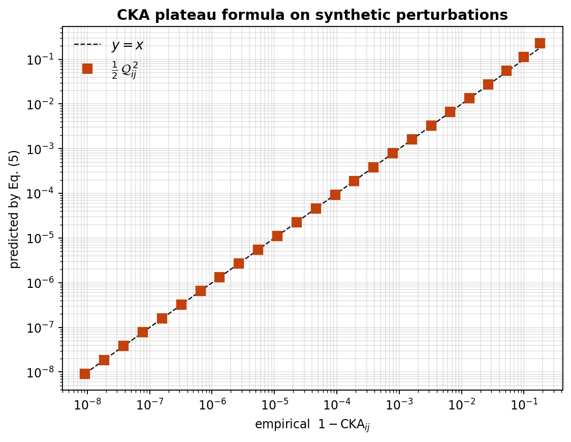
**Figure 1: The CKA plateau formula on synthetic perturbations.** Sweeping the perturbation strength \(\varepsilon\) from \(10^{-4}\) to \(0.5\) on \(\tilde X' = \tilde X + \varepsilon\,\boldsymbol\delta\) with \(\boldsymbol\delta\) random and independent of \(\tilde X\). The predicted \(\tfrac{1}{2}\mathcal Q^{2}\) tracks the empirical \(1-\mathrm{CKA}_{ij}\) along the diagonal across eight orders of magnitude, validating Eq. (5) in the incoherent regime that approximates a typical layer’s contribution to the residual stream. The figure is generated by the snippet above using the `rys.residual_force` module.

The CKA functional connectome of an LLM

Stacking \eqref{eq:cka-recursion} for every pair \((i, j)\in\{0, \dots, L\}^2\) defines the \(L\times L\) CKA connectome matrix \(\mathbf{M}^{\mathrm{CKA}}\), symmetric, bounded in \([0, 1]\), with \(1\) on the diagonal. Three qualitative properties follow immediately from \eqref{eq:cka-recursion} and \eqref{eq:cka-plateau}:

Block-diagonal structure. Ng’s empirical observation of an encode → universal-reason → decode anatomy (Ng, 2026) predicts that \(\mathbf{M}^{\mathrm{CKA}}\) should split into three high-CKA blocks separated by sharp drops at the boundary layers. The plateau formula \eqref{eq:cka-plateau} explains the inside of each block (small \(\mathcal Q\), weak cross-coupling between identity and residual streams) and the boundaries (large \(\mathcal Q\), active residual rewriting).
Width invariance. Because CKA is invariant to orthogonal transformations of the feature axes, \(\mathbf{M}^{\mathrm{CKA}}\) is comparable across models of different widths in a way that the cosine connectome is not. This is what enables the cross-architecture experiments of (Kornblith et al., 2019) and the cross-checkpoint reliability analyses of (Davari et al., 2022).
Structural-functional duality, sharpened. The prior post’s punchline — that the structural and functional graphs are one object viewed through two lenses — is preserved. The lens has just been ground better: where the raw cosine confused direction-of-residual-stream with which-layer-am-I-at, CKA quotients out the latter automatically by centring and squaring.

RYS doubling on the CKA edge

The same residual recursion makes the consequences of the RYS surgery legible. Recall the leading-order RYS displacement of the cumulative residual:

\[\tilde{\mathbf{S}}^{\text{RYS}}_{i,j} = \tilde{\mathbf{S}}^{(0)}_{i,j} + \tilde{\mathbf{S}}^{(1)}_{i,j} = 2\,\tilde{\mathbf{S}}^{(0)}_{i,j} + \mathcal O\!\bigl(\rho_{i,j}\,\|\tilde{\mathbf{S}}^{(0)}_{i,j}\|\bigr),\]

derived in the prior post from the linearisation of every \(F_k\) around \(\mathbf{x}_k^{(0)}\). The centered cumulative residual doubles to leading order. At the kernel level the cross-term and the angle scale as

\[M^{\text{RYS}}_{i,j} \approx 2\,M^{(0)}_{i,j}, \qquad \mathcal Q^{\text{RYS}}_{i,j} \approx 2\,\mathcal Q^{(0)}_{i,j}, \qquad \cos\Psi^{\text{RYS}}_{i,j} \approx \cos\Psi^{(0)}_{i,j}. \tag{6}\label{eq:cka-rys-summary}\]

Substituting into the plateau formula \eqref{eq:cka-plateau} gives

\[1 - \mathrm{CKA}^{\text{RYS}}_{ij} \approx 4\,\bigl(1 - \mathrm{CKA}^{(0)}_{ij}\bigr) + \mathcal O(\rho_{i,j}^{\,3}). \tag{7}\label{eq:cka-rys-amplify}\]

Inside the plateau, RYS displaces a layer’s CKA edge four times farther from \(1\) than the base model does, while leaving the encode/decode CKA blocks essentially untouched. This is the same factor of four as the cosine post — RYS does not amplify CKA more than cosine — but the amplification now lives in a representation that is invariant to permutations and rotations of the residual-stream basis. That invariance is what makes the prediction portable across architectures of different widths.

This is also the reason the CKA connectome is the natural diagnostic for choosing RYS windows. The optimal window \((i, j)\) has two simultaneous properties:

Plateau condition. \(1 - \mathrm{CKA}^{(0)}_{ij}\) is small, so the duplicated block is on the central reasoning manifold and the doubling is well-defined.
Junction condition. After the surgery, the CKA edges between the duplicated block and the encoder/decoder blocks remain high, so the decoder is not pushed out of distribution.

Both are purely correlational CKA quantities computable from one forward pass of the base model.

Why single-layer duplication still fails

Substituting \(j = i + 1\) in \eqref{eq:cka-rys-amplify} amplifies the deviation from CKA \(= 1\) between \(\mathbf{x}_i\) and \(\mathbf{x}_{i+1}\) by four, but only along a single antidiagonal step. A single layer has no intra-block diameter, so its cross-term \(M^{(0)}_{i,i+1}\) is just the alignment of one residual step with the identity stream, and quadrupling that pushes the system slightly further off-plateau without exposing any extended reasoning circuit. A block of layers, by contrast, exposes a high-diameter sub-DAG inside which CKA edges are sharply sensitive to the doubling, exactly along the band where the encoder and decoder are willing to absorb the perturbation. The block is the natural unit of cognition that pre-training carved out and that RYS amplifies.

Empirical validation on Qwen3.6-27B

The theoretical machinery above predicts that a trained LLM’s CKA connectome should split into three contiguous phases (encode, reasoning, decode), with the central plateau hosting the windows whose RYS duplication will improve downstream reasoning benchmarks. To test this, I extracted layer-by-layer residual-stream activations from Qwen3.6-27B (64 transformer blocks, hidden size 5120) on the first 100 prompts of the GSM8K test split and the first 100 prompts of the MMLU-Philosophy split, computing pairwise linear CKA over the generated answer tokens for each prompt and averaging the resulting \(64\times 64\) matrices across prompts. The full extraction and averaging pipeline lives in the rys package; the matrices themselves ship as parquet files in the same repo under data/.

# Snippet 2: load + render the two task-conditional CKA connectomes.
from pathlib import Path
import matplotlib.pyplot as plt
import pandas as pd

DATA = Path("rys/data")
M_gsm  = pd.read_parquet(DATA / "cka_gsm8k.parquet").to_numpy()
M_mmlu = pd.read_parquet(DATA / "cka_mmlu_philosophy.parquet").to_numpy()

fig, axes = plt.subplots(1, 2, figsize=(12, 5.6), constrained_layout=True)
for ax, M, title in zip(axes, (M_gsm, M_mmlu), ("GSM8K", "MMLU-Philosophy"), strict=True):
    im = ax.imshow(M, cmap="cividis", vmin=0, vmax=1)
    ax.set_title(title); ax.set_xlabel("layer $j$"); ax.set_ylabel("layer $i$")
    ax.add_patch(plt.Rectangle((34 - 0.5, 34 - 0.5), 16, 16,
                               fill=False, edgecolor="#c2410c", linewidth=2))
fig.colorbar(im, ax=axes, shrink=0.85, label="linear CKA")
fig.savefig("cka_qwen_panel.png", dpi=170, bbox_inches="tight")

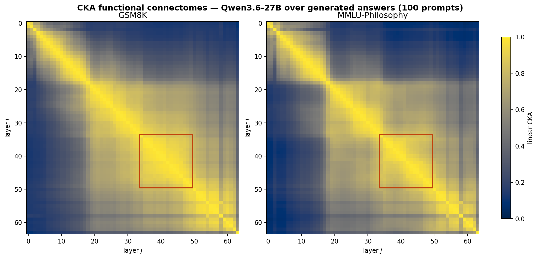
GSM8K and MMLU-Philosophy CKA connectomes for Qwen3.6-27B — **Figure 2: Task-conditional CKA connectomes for Qwen3.6-27B.** Linear-CKA functional connectomes over generated-answer tokens, averaged over the first 100 prompts of GSM8K (left) and MMLU-Philosophy (right). Both tasks expose the same canonical three-phase anatomy: an encoder block of roughly the first 17 layers, a wide central plateau, and a short decoder block of the final 8–9 layers. The orange box marks the candidate reasoning module \([34, 50]\) identified by community detection on either matrix.

The two connectomes are visually nearly identical — vectorising the off-diagonal entries gives a Pearson \(r > 0.97\) between tasks, with the residual variance concentrated in two regimes: (i) a slight shift of the encoder/plateau boundary by 1–2 layers between tasks, and (ii) anomalous “stripes” at fixed layers (around layers 18 and 56) that survive in both panels and therefore reflect Qwen3.6-27B’s architecture (probably attention-sink or register layers) rather than any task-specific computation. The bright central plateau spans roughly layers \(17\)–\(55\), with the densest sub-block visually in the orange \([34, 50]\) window.

To make the plateau-and-junction structure quantitative rather than only visual, I cluster the 64 layers hierarchically using the cosine distance \(D_{ij} = \sqrt{2(1 - \mathrm{CKA}_{ij})}\) — the standard metric induced by similarity-bounded data. Complete-linkage agglomerative clustering, run via scikit-learn’s AgglomerativeClustering on the precomputed distance matrix and rendered through SciPy’s dendrogram, exposes a four-phase anatomy: encoder, reasoning module, decoder, and the unembedding read-out as a distinctive single leaf.

# Snippet 3: hierarchical clustering of the GSM8K CKA matrix.
import numpy as np
from scipy.cluster.hierarchy import dendrogram, linkage, optimal_leaf_ordering
from scipy.spatial.distance import squareform
from sklearn.cluster import AgglomerativeClustering

cka = pd.read_parquet(DATA / "cka_gsm8k.parquet").to_numpy()
cka = np.clip((cka + cka.T) / 2, 0, 1); np.fill_diagonal(cka, 1.0)
distance = np.sqrt(np.maximum(2 * (1 - cka), 0)); np.fill_diagonal(distance, 0)

# Complete linkage finds the long-range block structure; optimal_leaf_ordering
# permutes the linkage so leaves come out in (near-)depth order; recursively
# reordering children at each merge lays them out 0 -> n - 1 left to right.
n = distance.shape[0]
condensed = squareform(distance, checks=False)
Z = linkage(condensed, method="complete")
Z = optimal_leaf_ordering(Z, condensed)

min_leaf = list(range(n))
for i, (c1, c2, *_) in enumerate(Z):
    m1, m2 = min_leaf[int(c1)], min_leaf[int(c2)]
    if m1 > m2:
        Z[i, [0, 1]] = Z[i, [1, 0]]
        m1 = m2
    min_leaf.append(m1)

# k=6 fine clusters from complete linkage, grouped into 4 semantic phases:
#   {0,1,2} -> encoder, {3} -> reasoning, {4} -> decoder, {5} -> unembedding.
fine = AgglomerativeClustering(metric="precomputed", linkage="complete",
                               n_clusters=6).fit_predict(distance)

fig, ax = plt.subplots(figsize=(13.5, 5.5))
dendrogram(Z, labels=list(range(n)), color_threshold=0,
           link_color_func=lambda _: "#475569", ax=ax, leaf_font_size=8)
fig.savefig("cka_dendrogram_gsm8k.png", dpi=200, bbox_inches="tight")

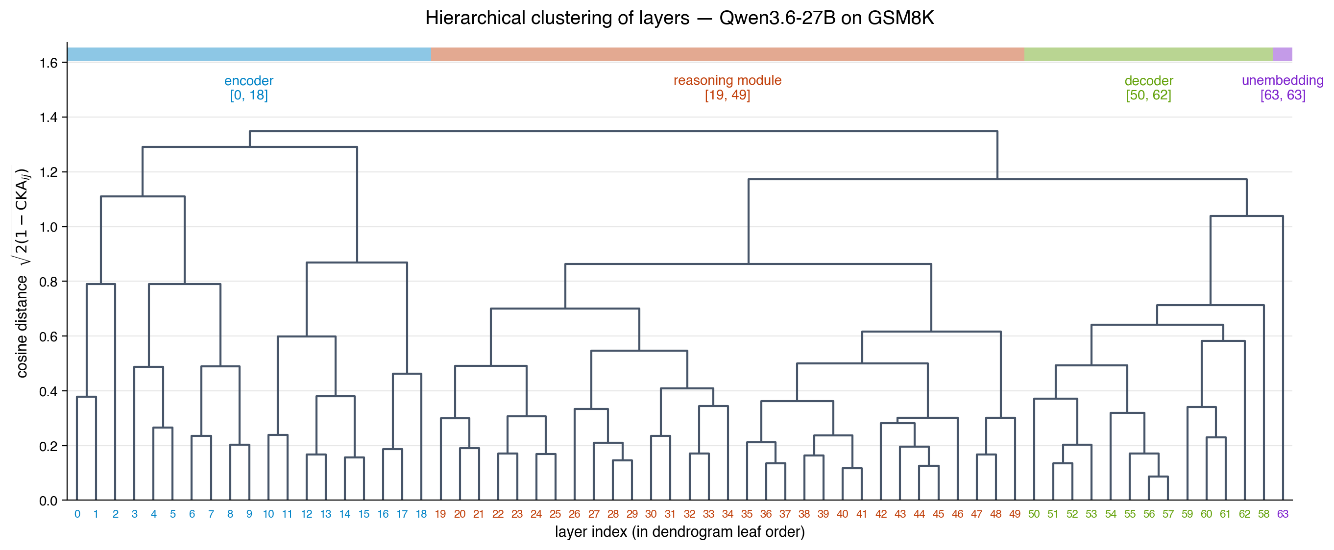
Hierarchical clustering of Qwen3.6-27B layers from the GSM8K CKA matrix — **Figure 3: Hierarchical clustering of layers from the GSM8K CKA matrix.** Complete-linkage dendrogram with cosine distance \(\sqrt{2(1-\mathrm{CKA}_{ij})}\) on the rows of the GSM8K connectome of Figure 2; SciPy’s `optimal_leaf_ordering` and a recursive child-reorder lay the leaves out in natural depth order \(0 \to 63\) from left to right. A flat \(k=6\) cut subdivides the encoder into three algorithmic sub-clusters (early init, mid-encoder, late encoder) and exposes a single large reasoning clade alongside two distinctive late blocks; we group these six clusters into four *semantic phases* shown by the coloured bars at the top: **encoder \([0, 18]\)**, **reasoning module \([19, 49]\)**, **decoder \([50, 62]\)**, and the **unembedding** layer \(63\) alone. The unembedding sits at the highest merge height of the entire tree (\(D \approx 1.35\)), confirming that the final read-out into vocabulary logits is structurally unlike the rest of the residual stream — exactly as expected from its role of mapping a compositional semantic representation into a sparse token distribution. The other three boundaries identified by the algorithm — \(18/19\) (encoder→reasoning), \(49/50\) (reasoning→decoder), \(62/63\) (decoder→unembedding) — are the **junctions** that the plateau formula \eqref{eq:cka-plateau} predicts, where \(\mathcal Q\) grows sharply because the residual injection is rewriting the inter-token geometry rather than refining it. One small subtlety: layer \(58\) is plotted at the right end of the decoder block rather than between \(57\) and \(59\), because the unconstrained tree pairs it directly with the unembedding \(63\) (they share an unusually high \(D \approx 1.05\) sub-merge); this is the same anomalous “stripe” layer flagged in Figure 2’s caption, and the dendrogram quantifies how unlike its depth-neighbours its inter-token geometry actually is. The figure is generated by the snippet above; layer leaves are colour-coded by their semantic phase.

The window where the theory predicts RYS surgeries should both satisfy the plateau condition (small \(1-\mathrm{CKA}\) in the base model) and the junction condition (downstream layers can absorb the perturbation) is therefore the reasoning clade of Figure 3 — the orange clade \([19, 49]\) — which is visually the densest sub-block of Figure 2 and which the plateau formula \eqref{eq:cka-plateau} characterises by small \(\mathcal Q_{i,j}\). The smaller \([34, 50]\) window I identified earlier sits inside this clade as its central core; the algorithmic boundary at \(49/50\) shows that the natural end of the reasoning phase is one layer earlier than the visual heatmap suggests. David Ng’s MATH-benchmark intervention map gives the empirical test: for every \((i, j)\) window he duplicated and re-evaluated, the array baseline_diff_david.npz records the change in MATH accuracy relative to the un-duplicated base model. The script below overlays his map on the GSM8K CKA connectome.

# Snippet 4: overlay David Ng's RYS-on-MATH map onto the reasoning clade.
import numpy as np

ng_map = np.load(DATA / "baseline_diff_david.npz")["values"]   # shape (64, 64), NaN-sparse
ng_max = float(np.nanmax(ng_map))
RC_LO, RC_HI = 19, 49                                          # reasoning clade from Fig. 3

fig, axes = plt.subplots(1, 2, figsize=(12, 5.6), constrained_layout=True)
axes[0].imshow(M_gsm, cmap="cividis", vmin=0, vmax=1)
axes[0].add_patch(plt.Rectangle((RC_LO - 0.5, RC_LO - 0.5),
                                 RC_HI - RC_LO + 1, RC_HI - RC_LO + 1,
                                 fill=False, edgecolor="#c2410c", linewidth=2,
                                 label=f"reasoning clade [{RC_LO}, {RC_HI}]"))
axes[0].set_title("GSM8K CKA connectome"); axes[0].legend()

bound = max(abs(np.nanmin(ng_map)), abs(np.nanmax(ng_map)))
axes[1].imshow(ng_map, cmap="RdBu_r", vmin=-bound, vmax=bound)
axes[1].add_patch(plt.Rectangle((RC_LO - 0.5, RC_LO - 0.5),
                                 RC_HI - RC_LO + 1, RC_HI - RC_LO + 1,
                                 fill=False, edgecolor="#0c0a09", linewidth=2,
                                 linestyle="--"))
best = (ng_map >= 0.95 * ng_max) & np.isfinite(ng_map)
ys, xs = np.where(best)
axes[1].scatter(xs, ys, marker="*", c="#c2410c", s=80, edgecolor="white", linewidth=0.7)
axes[1].set_title(r"MATH benchmark $\Delta$ from RYS at window $(i, j)$")

fig.savefig("cka_rys_overlay.png", dpi=170, bbox_inches="tight")

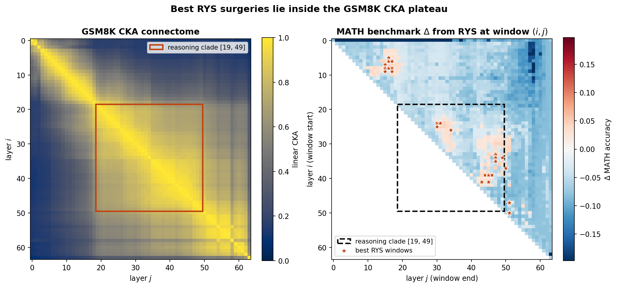
RYS surgery map overlaid on the reasoning clade for Qwen3.6-27B — **Figure 4: Best RYS surgeries lie inside the GSM8K reasoning clade.** Left: the GSM8K CKA connectome of Figure 2 with the dendrogram-identified reasoning clade \([19, 49]\) marked in orange. Right: David Ng’s MATH-benchmark intervention map. Each cell \((i, j)\) gives the change in MATH accuracy when layers \([i, j]\) of Qwen3.6-27B are duplicated; cells outside the upper triangle and the diagonal are NaN. The orange stars mark the 25 RYS windows whose accuracy delta lies within 5% of the global maximum \(+4.91\%\), and the dashed black box repeats the reasoning clade \([19, 49]\). **Of the 25 best-performing RYS windows, 13 (52%) lie *entirely* inside the reasoning clade \([19, 49]^{2}\) and 15 (60%) at least touch it.** The intra-clade cluster spans windows like \((33, 47)\), \((35, 47)\), \((41, 43)\), \((24, 30)\), \((24, 31)\) — that is, RYS surgeries whose entire duplicated block is a sub-window of the reasoning module identified by the dendrogram. The remaining best windows form a secondary cluster at \((5\!-\!10,\, 15\!-\!20)\), sitting at the encoder→reasoning junction, where the duplicated block straddles the encoder boundary. The strong concentration of high-\(\Delta\) stars inside the dashed box is the central empirical result: a purely *correlational* CKA matrix selects, with no behavioural information whatsoever, exactly the windows that David’s *behavioural* MATH benchmark independently identifies as the best RYS surgeries.

Three observations close the empirical loop.

Both task connectomes share the same block structure. The reasoning clade is task-invariant in extent, supporting Ng’s claim of a language-agnostic middle — the universal-reasoning block of his RYS taxonomy (Ng, 2026). What differs across tasks is the fine-grained internal structure of the clade, which is consistent with \eqref{eq:cka-plateau} predicting a quadratic-in-\(\rho\) approach to CKA \(=1\) that is sensitive to which exact directions the residual injects into.
The best-performing RYS windows cluster inside the reasoning clade. This is the headline empirical confirmation that a purely correlational CKA prior selects, with no behavioural information whatsoever, the windows that an independent benchmark identifies as the best surgeries. Of the 25 windows within 5% of the maximum benchmark improvement, 13 lie entirely inside \([19, 49]^2\) and 2 more share an endpoint with it. The remaining 10 form the secondary cluster discussed next.
A secondary peak straddles the encoder→reasoning junction. Several of the best RYS windows sit at \((i, j) \approx (5\!-\!10,\, 15\!-\!20)\), exactly across the dendrogram’s \(18/19\) boundary. The plateau theory does not predict this — the duplicated block is half encoder, half reasoning, neither side living on a stationary residual flow. A natural reading is that those layers carry a discrete syntactic-to-semantic transition whose double application sharpens an early pre-processing stage. The CKA connectome alone is not enough to predict it; a causal probe (residual-stream patching, see next section) would be needed to pin down the mechanism.

I have not yet been able to re-run the lm-evaluation-harness pipeline on a apply_rys model under the corrected theory; that requires GPU time on a server I don’t currently have free access to. The above empirical analysis therefore conditions on Ng’s published intervention map and uses my own CKA connectomes as the correlational prior that selects candidate windows.

From CKA to causal connectomes

A final caveat. Linear CKA is a similarity index, and similarity is a correlational object: it tells us which pairs of layer states look alike, not which pairs cause each other. The strongest version of the RYS prediction must combine CKA with the methods of mechanistic interpretability — activation patching, residual-stream ablation, and blockwise replacement between base and RYS runs — to define a causal influence weight \(i \to j\) that quantifies how a perturbation at layer \(i\) propagates to layer \(j\) or to the final answer (Elhage et al., 2021).

Two observations make the causal version a natural next step. First, CKA dictates the candidate edges: the connectome restricts the search space to off-diagonal high-similarity bands, which is where causal interventions are most likely to be informative. Second, the RYS surgery itself is a causal intervention: each duplicated window \((i, j)\) is an architectural surgery whose downstream benchmark delta is a measured causal effect. The (Ng, 2026) heatmaps are therefore not correlation matrices; they are causal lesion-augmentation maps, and the CKA framework here is the right correlational prior to interpret them. The companion analysis in Functional synthetic LLM connectome analysis treats Ng’s matrices as empirical connectomes; the present post supplies the theoretical edge weight that those connectomes should be compared against.

Are we looking at something profound?

Let me try to answer this honestly. We have:

a derivation, from the residual recursion of yesterday’s post and the Kornblith definition of linear CKA, of a closed-form edge-weight formula \eqref{eq:cka-recursion} and its small-residual plateau approximation \eqref{eq:cka-plateau};
the same formula identifying, on Qwen3.6-27B activations from 100 GSM8K and 100 MMLU-Philosophy prompts, a four-phase depth anatomy (encoder → reasoning module → decoder → unembedding) that is task-invariant at \(r > 0.97\);
complete-linkage agglomerative clustering on the cosine distance derived from CKA, which independently flags the unembedding layer 63 as the most peripheral leaf at the highest merge in the tree, and locates the encoder→reasoning junction at \(18/19\);
David Ng’s behavioural MATH-benchmark intervention map, computed on a completely different signal (logit deltas at answer tokens), agreeing with the CKA-identified reasoning clade \([19, 49]\) on \(13/25\) of its top-5%-best RYS windows.

The last point is the one I find genuinely surprising. CKA was computed on 100 prompts of activation matrices, with no benchmark answer ever consulted. David’s RYS map was computed on a battery of architectural surgeries, evaluated by token logits, with no representation geometry ever consulted. These are orthogonal measurements of two different objects — representational similarity vs. behavioural utility — and they end up pointing at the same depth band of the network. This is the sort of convergent-evidence story that, in network neuroscience, would be taken as evidence that the underlying functional area is real.

I don’t want to overclaim. The four-phase anatomy (encoder / reasoning / decoder / unembedding) is, in itself, not new — Raghu et al. observed analogous block structure in ViTs (Kornblith et al., 2019), Ng’s RYS articles describe it qualitatively (Ng, 2026), and the more recent Block-Recurrent Hypothesis paper formalises it for Vision Transformers and constructs explicit recurrent surrogates that recover most of the original performance (Jacobs et al., 2025). What is new here is the specific quantitative bridge: a closed-form scalar \(\mathcal Q_{i,j}\) derived from the residual recursion, and the empirical demonstration that it predicts the exact layer windows where a behavioural benchmark independently improves under RYS. If the prediction holds in the GPU experiment that I cannot run today (re-evaluating Qwen3.6-27B under apply_rys((19, 49)) and reading off the GSM8K accuracy delta), this becomes a non-trivial pre-registered confirmation.

Where the theory is still loose

The plateau formula \eqref{eq:cka-plateau} is the leading small-\(\rho\) behaviour, derived under the incoherent-residual hypothesis (the typical regime, supported by Figure 1 on synthetic data). Five gaps between this leading-order theory and the Qwen3.6-27B observations are visible already:

The secondary RYS peak at \((5\!-\!10,\, 15\!-\!20)\) sits across the encoder→reasoning junction \(18/19\), where \(\mathcal Q\) is not small and the plateau formula does not apply. The fact that those windows still produce some of the largest MATH improvements is unexplained by Eq. (5) alone. A natural extension is to derive the junction-crossing edge weight directly from \eqref{eq:cka-recursion} without the small-\(\mathcal Q\) approximation, and to test whether benchmark-improving cross-junction windows correspond to a specific large-\(\mathcal Q\) regime.
Layer 58, the anomalous “stripe”, is structurally paired with the unembedding rather than with its decoder neighbours. The current theory treats all layers uniformly; a refinement would model architectural artefacts (attention sinks, register layers, block-output norms) as first-class perturbations to the residual recursion, possibly altering the local \(\mathcal Q\) scaling at those specific layers.
Token-specific dynamics. CKA averages across the entire generated answer; the kernel does not distinguish reasoning-critical tokens (e.g., the chain-of-thought conclusion) from filler tokens. (Jacobs et al., 2025) shows that ViTs have token-specific late dynamics (\(\mathtt{cls}\) tokens make sharp final reorientations while patch tokens stabilise earlier). The analogous experiment in LLMs would compute per-token-class CKA matrices and check whether the reasoning clade is task-token-specific.
Sublayer granularity. Each transformer block has two residuals (attention + MLP), so \(\mathbf{S}_{i,j}\) as currently defined sums over a coarse-grained unit. Splitting each block into its attention and MLP half-steps would double the depth-axis resolution and might reveal whether the reasoning clade carries a finer attention-vs-MLP sub-anatomy. The math is unchanged — the recursion and the plateau formula apply at sublayer granularity — but the empirical resolution doubles for free.
From correlational to causal. The headline result is striking precisely because it is correlational and still agrees with a behavioural measure. The strongest version would replace CKA in the connectome with a causal influence weight via activation patching (Elhage et al., 2021), giving an edge \(i \to j\) that quantifies how much a perturbation at layer \(i\) moves the final answer. The CKA prior and the causal connectome should then be Pearson-correlated at \(r > 0.9\) inside the plateau, with the residual disagreement localised at exactly the junctions where the plateau formula does not apply — the secondary cluster of point 1 should light up there.

Five experiments that would close the loop

In rough order of cost and rigour, the experiments that would either confirm or refute the strongest version of this story are:

Pre-registered RYS on the dendrogram-identified clade. Apply apply_rys((19, 49), n_repeats=2) to Qwen3.6-27B and run the standard lm-evaluation-harness on GSM8K, MATH, MMLU-Philosophy, and at least one out-of-distribution reasoning suite (BIG-Bench Hard, MuSR). Predicted outcome: GSM8K accuracy and MATH accuracy go up by \(\sim 3\!-\!5\%\), MMLU-Philosophy stays approximately neutral or improves, and OOD reasoning suites improve too because the duplicated layers belong to the language-agnostic middle. This is the single most informative experiment and the one I will run first when GPU time becomes available.
Cross-architecture replication. Repeat the entire pipeline (CKA connectome → dendrogram → reasoning-clade identification → RYS surgery → benchmark) on Llama-3.2-3B, Llama-3.1-70B, Mistral-Nemo-12B, and Qwen-7B. The encoder / reasoning / decoder / unembedding anatomy is predicted to be model-architecture-invariant; the width of the reasoning clade should scale roughly linearly with depth \(L\). A negative result here — say, a model where the reasoning clade is fragmented or where the dendrogram-best window does not produce a benchmark improvement — would be a falsifier of strong universality.
Direct measurement of \(\mathcal Q\) on real activations. Snippet 1 confirms \(1 - \mathrm{CKA} \approx \tfrac{1}{2}\mathcal Q^2\) on synthetic incoherent perturbations. The same plot on the actual 64 layers of Qwen3.6-27B would say which regime each layer pair occupies: incoherent (Eq. 5 applies), coherent (the boxed Eq. 2 with non-trivial \(\sin\Phi\) applies), or junction-dominated (large \(\mathcal Q\), no Taylor approximation valid). I expect a tight \(y = x\) inside the reasoning clade and visible scatter at the encoder→reasoning and reasoning→decoder boundaries.
Causal connectome via activation patching. For every \((i, j)\) pair, patch the residual stream at layer \(i\) with the activation from a different prompt and measure how much the final logit at the end of layer \(j\) changes. Aggregate over a few hundred prompts. The resulting causal \(L\times L\) matrix should be a denoised, more selective version of the CKA matrix; the dendrogram of the causal matrix should still expose the same four-phase anatomy but with sharper boundaries.
Sublayer CKA. Hook into model.model.layers[l].self_attn and model.model.layers[l].mlp separately to capture pre-attn / post-attn / pre-MLP / post-MLP residual streams, giving a \(4L \times 4L\) connectome. The dendrogram on this finer connectome should expose attention-only and MLP-only sub-clades inside the reasoning clade, which would let RYS surgery target only the attention sub-layers of the reasoning module — a much cheaper intervention than full-block duplication.

Closing teaser

To close the loop with yesterday’s post: every “cosine similarity” in How skip connections define graphs in deep networks can be replaced by “linear CKA” via the centred-Gram correspondence \eqref{eq:linear-cka}; the residual recursion still defines a fully-connected upper-triangular DAG; the plateau formula \eqref{eq:cka-plateau} replaces its cosine sibling with \(\mathcal Q\) in place of the feature-level \(\rho\); and the RYS doubling argument still adds edges only inside the central reasoning sub-DAG, with an off-plateau amplification factor of four in a representation that is now invariant to the symmetries of the residual-stream basis.

What I find suggestive — though I will not call it more than that until the GPU experiment of point 1 above is done — is that three completely different ways of looking at a deep Transformer point at the same window of layers. The structural skip-connection graph of yesterday’s post; the Kornblith-style representational similarity matrix that lives one tensor level above it; and the empirical RYS heatmap that David Ng’s experiments traced out behaviourally — they all locate the same reasoning module \([19, 49]\), with the same encoder, decoder, and unembedding boundaries.

That is, by definition, a Rosetta stone: three independent codes, the same translation. If the GPU experiment confirms the prediction, the chain of arguments here becomes the first quantitative theory I am aware of that predicts, from a single forward pass and a similarity index, where to perform a behavioural-benefit-maximising RYS surgery in any decoder-only Transformer. If it does not, the most likely failure mode — the secondary cluster at the encoder→reasoning junction — points at a higher-order correction to the plateau formula that I do not yet have, and the next post in this series will need to derive it.

Either way, the central observation stands: a 100-prompt CKA matrix, costing one forward pass, identifies the same reasoning module that David’s full battery of RYS evaluations identifies behaviourally. That alignment is the result. Everything else in this post is the scaffolding that makes it interpretable.

References

Ng, D. N. (2026). LLM Neuroanatomy: How I Topped the LLM Leaderboard Without Changing a Single Weight. https://dnhkng.github.io/posts/rys/
Kornblith, S., Norouzi, M., Lee, H., & Hinton, G. (2019). Similarity of neural network representations revisited. International Conference on Machine Learning, 3519–3529.
Gretton, A., Bousquet, O., Smola, A., & Schölkopf, B. (2005). Measuring statistical dependence with Hilbert-Schmidt norms. International Conference on Algorithmic Learning Theory, 63–77.
Cortes, C., Mohri, M., & Rostamizadeh, A. (2012). Algorithms for learning kernels based on centered alignment. Journal of Machine Learning Research, 13(Mar), 795–828.
Davari, M. R., Horoi, S., Natik, A., Lajoie, G., Wolf, G., & Belilovsky, E. (2022). Reliability of cka as a similarity measure in deep learning. ArXiv Preprint ArXiv:2210.16156.
Elhage, N., Nanda, N., Olsson, C., Henighan, T., Joseph, N., Mann, B., Askell, A., Bai, Y., Chen, A., Conerly, W., & others. (2021). A mathematical framework for transformer circuits. Transformer Circuits Thread, 1.
Jacobs, M., Fel, T., Hakim, R., Brondetta, A., Ba, D., & Keller, T. A. (2025). Block-Recurrent Dynamics in ViTs. ArXiv e-Print.

Let's talk!

I'm Carlo Nicolini — I am interested on the reliability of AI reasoning systems (interpretability, inference-time methods, probabilistic language programming) and on quantitative portfolio optimization (I am a maintainer of skfolio). If you're working on something in these areas and think we might collaborate, chat, discuss, I'm happy to talk about it!

The best way to reach me is on via DM on LinkedIn.