1. Question
The useful question is no longer whether a small recurrent model can beat a large dense MLP. That comparison is too easy to misread. The sharper question is:
If dense networks and fractal/recurrent networks are both shrunk aggressively, which family owns the validation/test Pareto frontier?
The objective is to reduce learned memory while spending more inference-time computation. The candidate mechanism is a fixed recurrent scaffold:
\[h_0=\phi(W_{\mathrm{in}}x), \qquad h_{t+1}=\phi\left(h_t+\phi(h_tG^\top)\right), \qquad \hat y=W_{\mathrm{out}}[x,h_T].\]Here $G$ is a fixed graph, often a Kronecker power of the Sierpinski initiator
\[K_0 = \begin{bmatrix} 1 & 1 \\ 1 & 0 \end{bmatrix}, \qquad G = K_0^{\otimes k}.\]The learned parameters live in the input projection and the readout. The recurrent graph contributes computation and inductive bias, not gradient-tracked storage.
This post rewrites the earlier experimental story around parameter frontiers. The old single-point results are useful historical context. The new results compare dense and fractal/reservoir models while shrinking both sides.
2. Why Brain-Inspired Recurrence?
Several biological motifs point toward this design.
Dentate gyrus and cerebellar expansion. Both systems use expansion and sparsification to separate inputs before downstream learning. In a machine-learning model, this suggests mapping low-dimensional inputs into a larger state and training only a small downstream readout.
CA3 recurrence and CA1 readout. Hippocampal CA3 is often modeled as an autoassociative recurrent network for pattern completion, while CA1 reads out and recodes the resulting activity (Jaeger, 2001; Maass et al., 2002; Lukoševičius & Jaeger, 2009). The best early improvement came from reading directly from the high-dimensional recurrent state instead of compressing it back to the input dimension.
Leaky and multi-timescale loops. Biological recurrence is not one clock. Leaky-integrator reservoirs and multiple-timescale recurrent networks motivate parallel fast/slow recurrent states (Yamashita & Tani, 2008).
Gated recurrent updates. Dendritic gating and recurrent highway networks motivate tiny learned gates over fixed recurrence (Guerguiev et al., 2017; Zilly et al., 2017):
\[\tilde h_{t+1}=\phi(h_t+\phi(h_tG^\top)), \qquad h_{t+1}=(1-z)h_t+z\tilde h_{t+1}.\]These ideas connect naturally to looped transformers, Universal Transformers, adaptive computation time, and equilibrium models, all of which trade repeated computation for stored parameters (Graves, 2016; Dehghani et al., 2019; Bai et al., 2019).
3. Graphs And Connectivity
The Kronecker graph is attractive because its spectrum factorizes exactly:
\[\operatorname{eig}(A\otimes B)=\{\lambda_i(A)\lambda_j(B)\}_{i,j}.\]That identity lets us set the spectral radius and reason about stability. It also produces self-similar adjacency patterns:
import numpy as np

def kronecker_adjacency(depth: int) -> np.ndarray:
    init = np.array([[1.0, 1.0], [1.0, 0.0]])
    graph = init.copy()
    for _ in range(depth - 1):
        graph = np.kron(graph, init)
    np.fill_diagonal(graph, 0.0)
    return (graph > 0).astype(float)
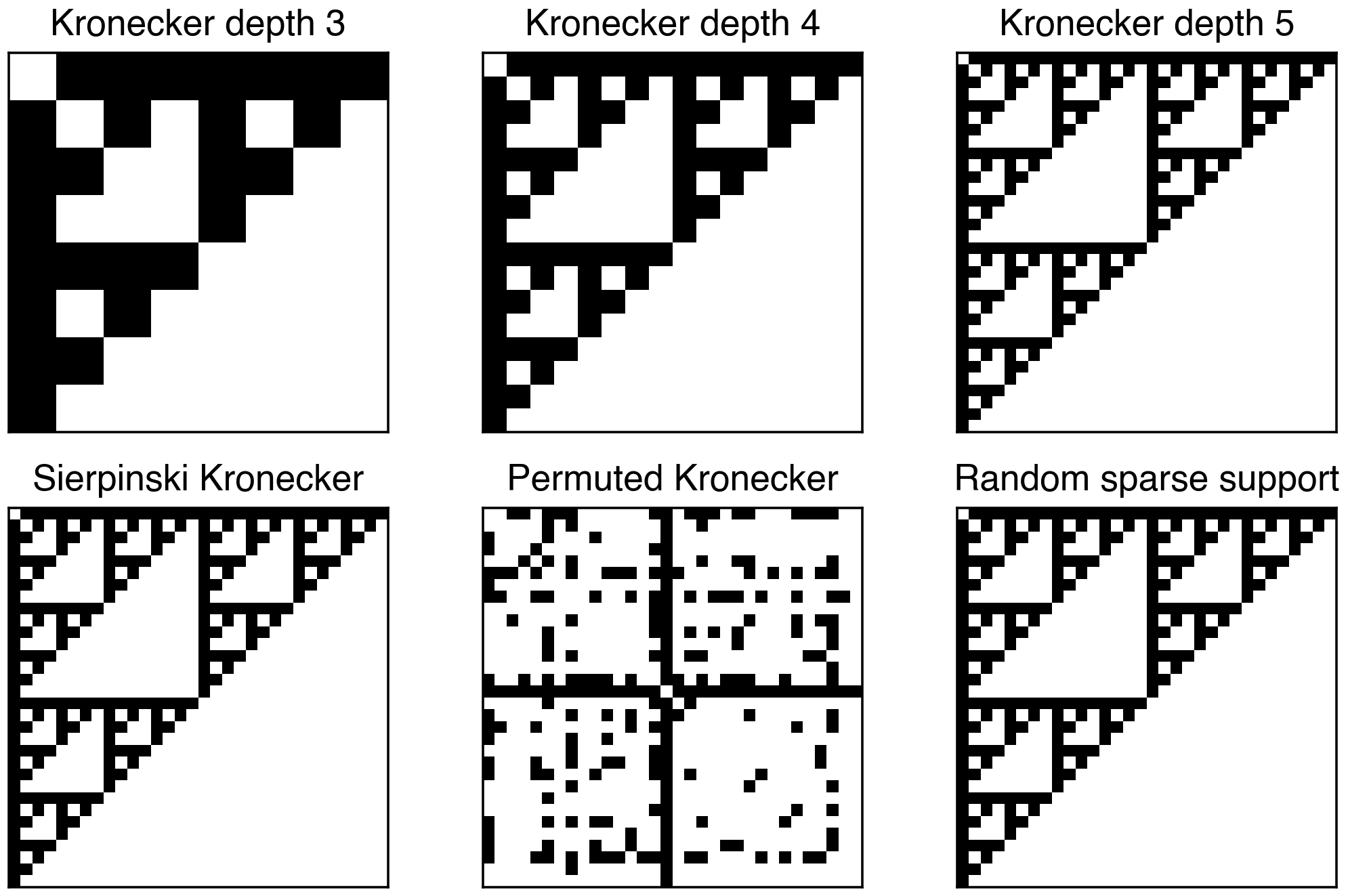
Figure 1. Kronecker/Sierpinski adjacency matrices and graph controls used in the frontier experiments.
The architecture used in the current frontier run is:
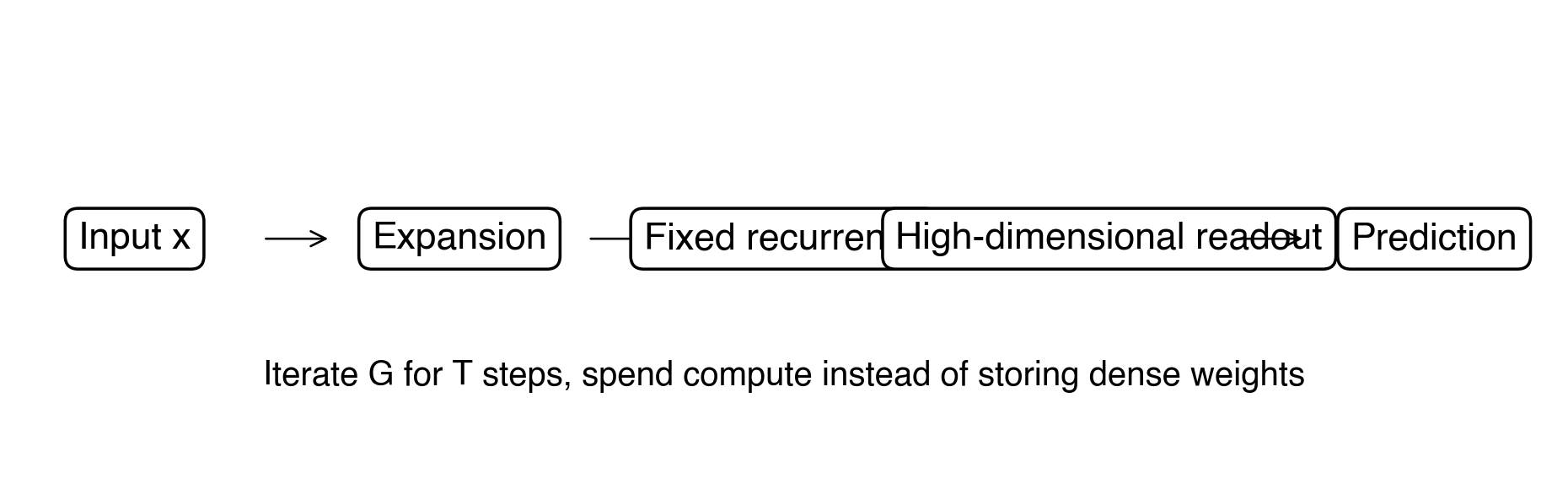
Figure 2. Expand, iterate a fixed graph, then read from the high-dimensional recurrent state.
4. Experimental Protocol
The new runner is experiments/multi_frontier.py. It supports regression, binary classification, and multiclass classification.
python experiments/multi_frontier.py \
  --compact \
  --datasets friedman1,sine,multiscale_fourier_regression,classification_20d,gaussian_quantiles,digits,synthetic_5class \
  --seeds 101,202,303,404,505
Every model reports raw and effective learned parameters. A Pareto point is non-dominated if no other model has both fewer learned parameters and a better validation score.
Families compared:
| Family | Description |
|---|---|
| Dense | ReLU MLP width sweep |
| Dense AdamW | same, with weight decay |
| Dense deep | deeper MLP controls |
| Kronecker reservoir | fixed Sierpinski/Kronecker recurrence |
| Gated Kronecker | scalar-gated fixed Kronecker recurrence |
| Random sparse reservoir | same density pattern class, random values |
| No recurrence | expansion plus readout without graph mixing |
Tasks:
| Group | Datasets |
|---|---|
| Regression | friedman1, sine, multiscale_fourier_regression |
| Binary classification | swiss_roll, circles, moons, s_curve_binary, gaussian_quantiles, classification_20d |
| Multiclass | iris, wine, digits, synthetic_3class, synthetic_5class |
The broad 14-dataset compact sweep used five seeds and quick epochs. A selected full compact sweep used five seeds on the most informative regression, binary, and multiclass datasets.
5. Regression Frontiers
Friedman1
The earlier single-point result suggested a Kronecker reservoir could beat large dense baselines. A dedicated parameter frontier made the picture clearer.
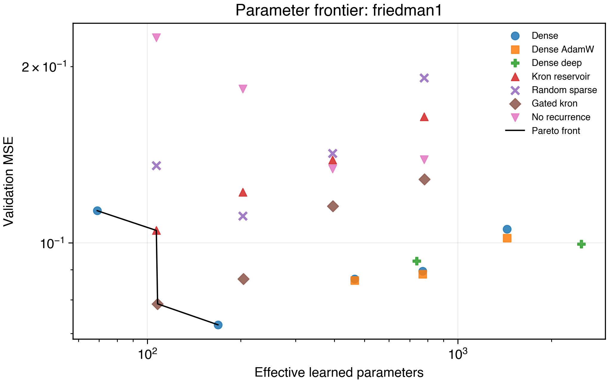
Figure 3. Friedman1 validation MSE versus effective learned parameters.
In the minimal five-seed frontier, the low-parameter recurrent model owned the best point:
| Model | Mean validation MSE | Effective parameters |
|---|---|---|
| Dense h=8 | 0.08822 | 169 |
| Dense h=16 | 0.06452 | 465 |
| Dense AdamW h=22 | 0.06014 | 771 |
| Kronecker reservoir H=16 | 0.05525 | 203 |
This is the strongest result so far. A 203-parameter recurrent scaffold beats dense models with two to four times more learned parameters.
The graph-control result is more nuanced:
| H=16 model | Mean validation MSE | Effective parameters |
|---|---|---|
| Random sparse reservoir | 0.05540 | 203 |
| Permuted Kronecker reservoir | 0.05770 | 203 |
| Dense-random reservoir | 0.05821 | 203 |
| Kronecker reservoir | 0.05830 | 203 |
| No recurrence | 0.07486 | 203 |
| Dense h=16 | 0.06452 | 465 |
Recurrence is doing useful work, because the no-recurrence control is much worse. Raw Kronecker topology is not yet uniquely superior at H=16; random sparse recurrence is slightly ahead in this control run.
Sine Regression
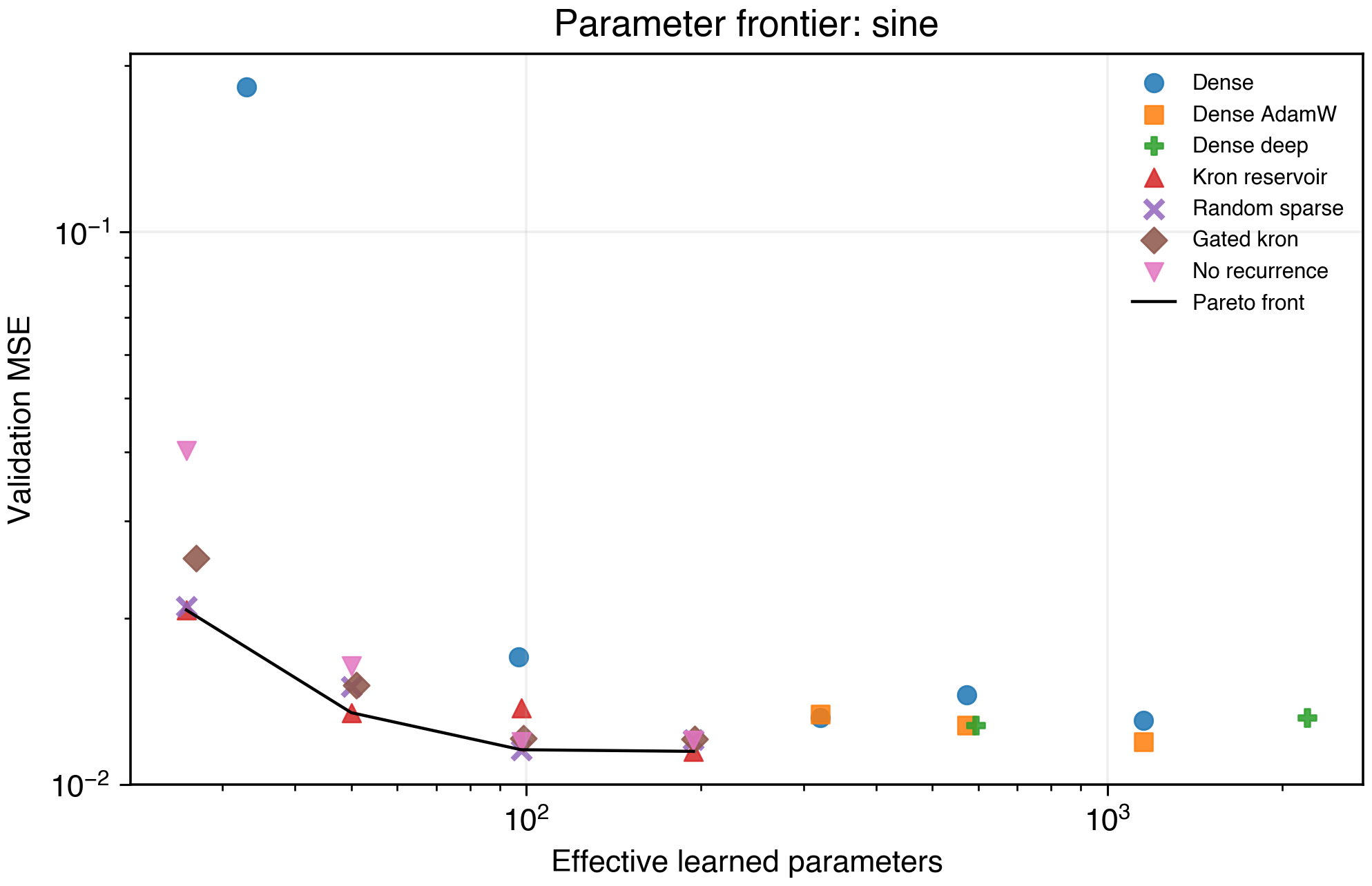
Figure 4. Sine regression frontier.
Sine regression strongly favors tiny recurrent reservoirs at low budgets:
| Model | Mean validation MSE | Effective parameters |
|---|---|---|
| Kronecker reservoir H=8 | 0.0207 | 26 |
| Kronecker reservoir H=16 | 0.0135 | 50 |
| Random sparse reservoir H=32 | 0.0116 | 98 |
| Kronecker reservoir H=64 | 0.0115 | 194 |
| Dense h=16 | 0.0253 | 321 |
| Dense deep h=32 | 0.0145 | 2,209 |
Here the memory reduction is clear. Small recurrent scaffolds provide a better low-parameter basis for smooth periodic structure than dense MLPs at comparable budgets.
Multiscale Fourier Regression
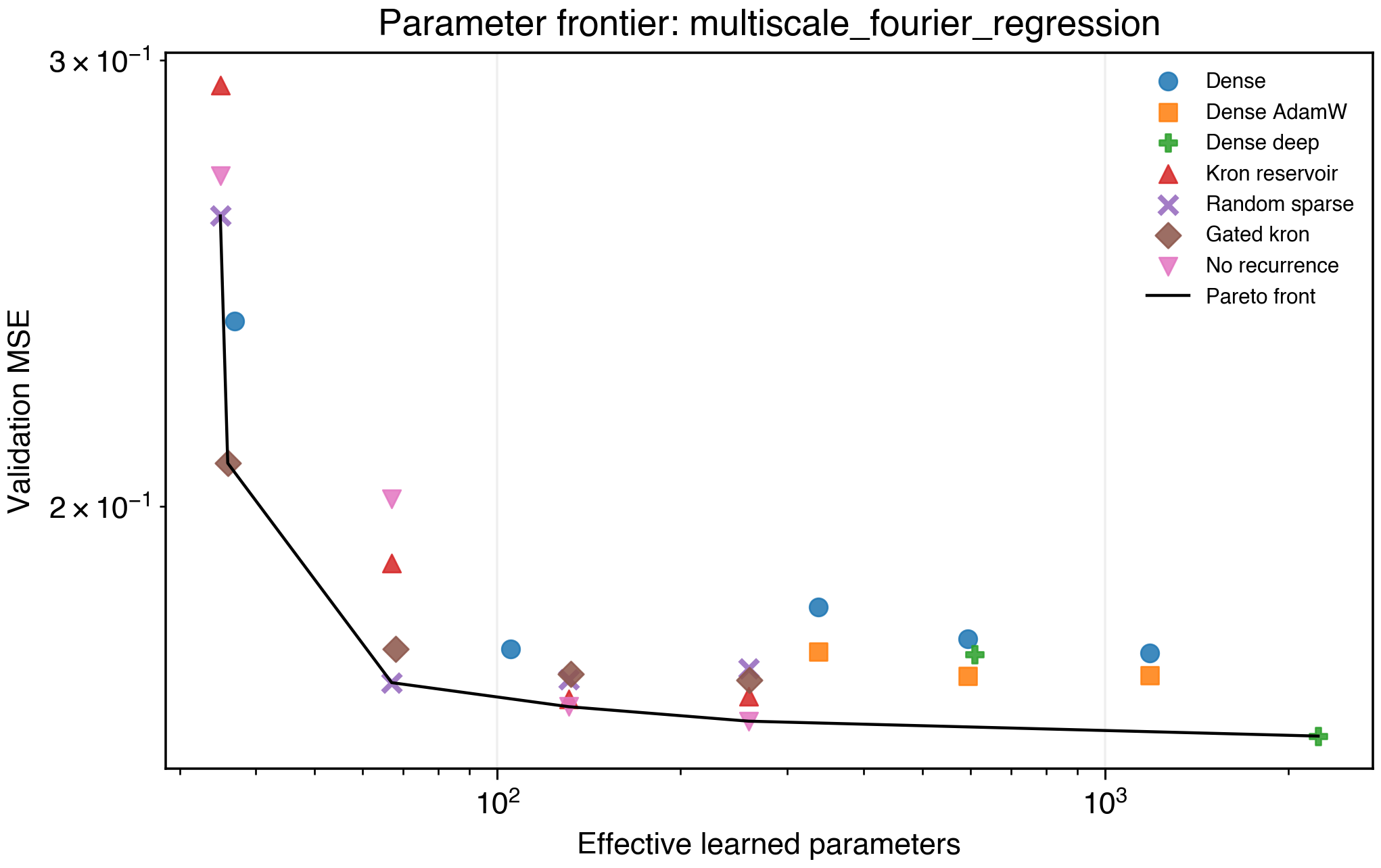
Figure 5. Multiscale Fourier regression frontier.
This task is harder. Random sparse and gated reservoirs dominate small budgets, while dense deep models recover at larger budgets:
| Model | Mean validation MSE | Effective parameters |
|---|---|---|
| Gated Kronecker H=8 | 0.2080 | 36 |
| Random sparse reservoir H=16 | 0.1703 | 67 |
| No-recurrence H=64 | 0.1645 | 259 |
| Dense deep h=32 | 0.1623 | 2,241 |
The result is a caution: recurrence helps at tiny budgets, but this high-frequency target also rewards larger dense capacity.
6. Binary Classification Frontiers
Low-dimensional binary tasks saturate quickly, but the small-budget region remains informative.
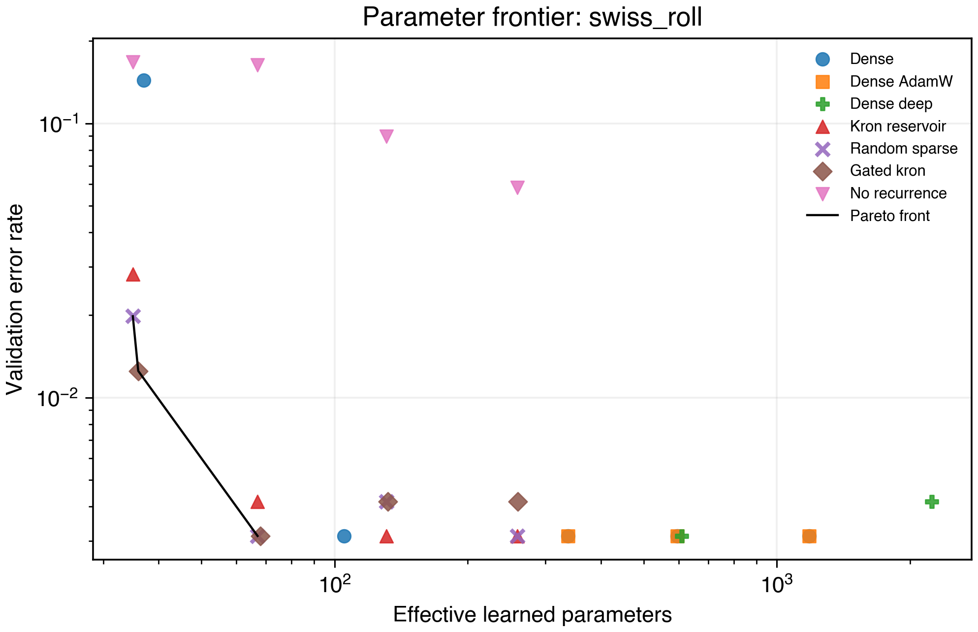
Figure 6. Swiss roll frontier.
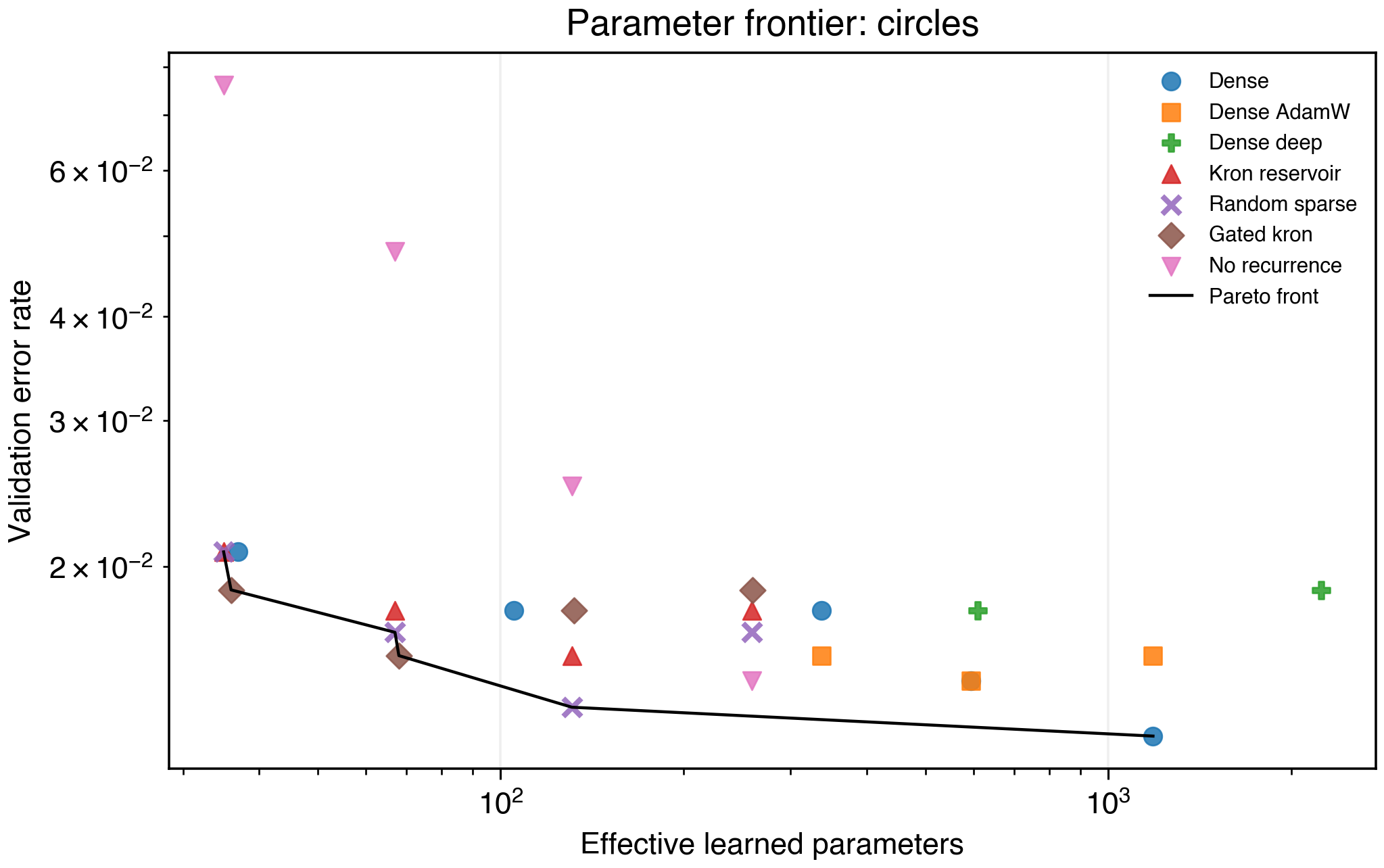
Figure 7. Circles frontier.
| Dataset | Low-parameter frontier owner | Effective parameters | Accuracy |
|---|---|---|---|
| Swiss roll | Gated Kronecker H=8 | 36 | 0.988 |
| Circles | Gated Kronecker H=8 | 36 | 0.981 |
| Moons | Kronecker H=8 | 35 | 0.972 |
| S-curve binary | Kronecker H=8 | 35 | 0.985 |
These are real low-memory wins, but the datasets are close to saturated. They are useful smoke tests, not the main evidence.
Harder binary tasks are less favorable:
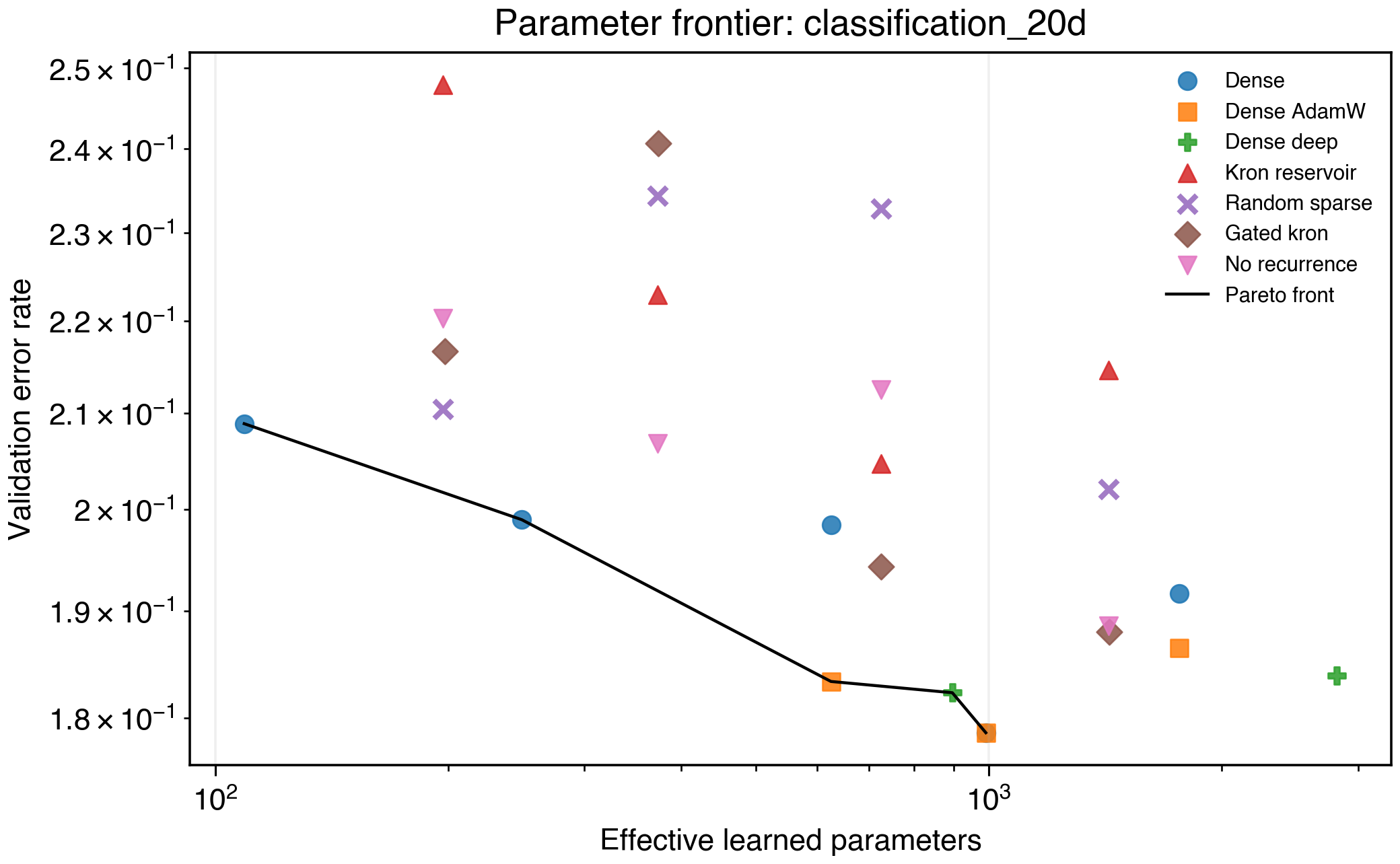
Figure 8. Higher-dimensional binary classification frontier.
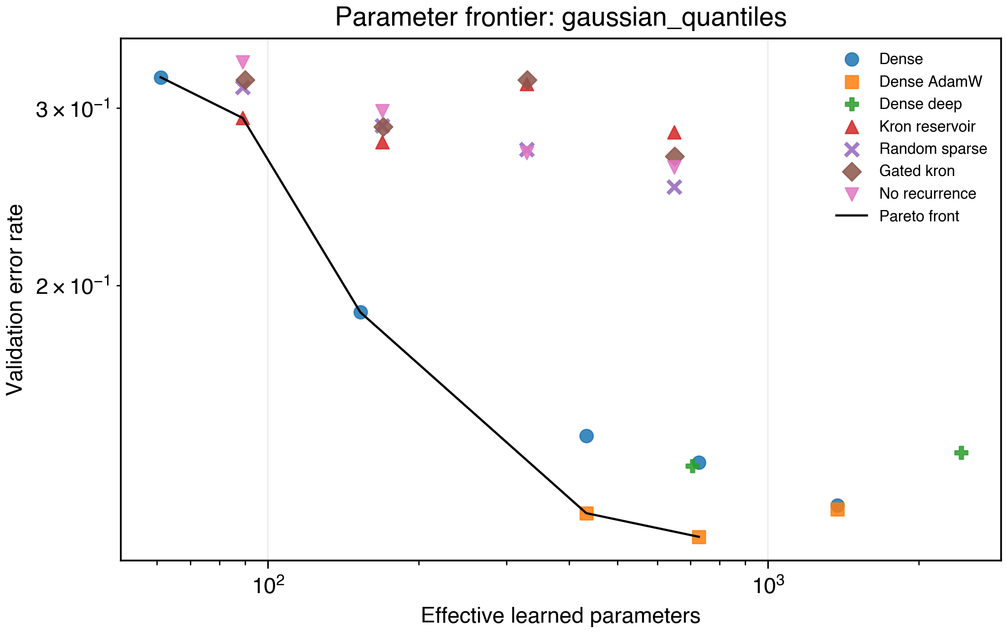
Figure 9. Gaussian quantiles frontier.
On classification_20d, dense MLPs own the Pareto frontier. On gaussian_quantiles, Kronecker H=8 improves over tiny dense h=4, but dense baselines dominate once they reach h=8 and above. This suggests the current reservoir needs better input feature construction for higher-dimensional classification.
7. Multiclass Frontiers
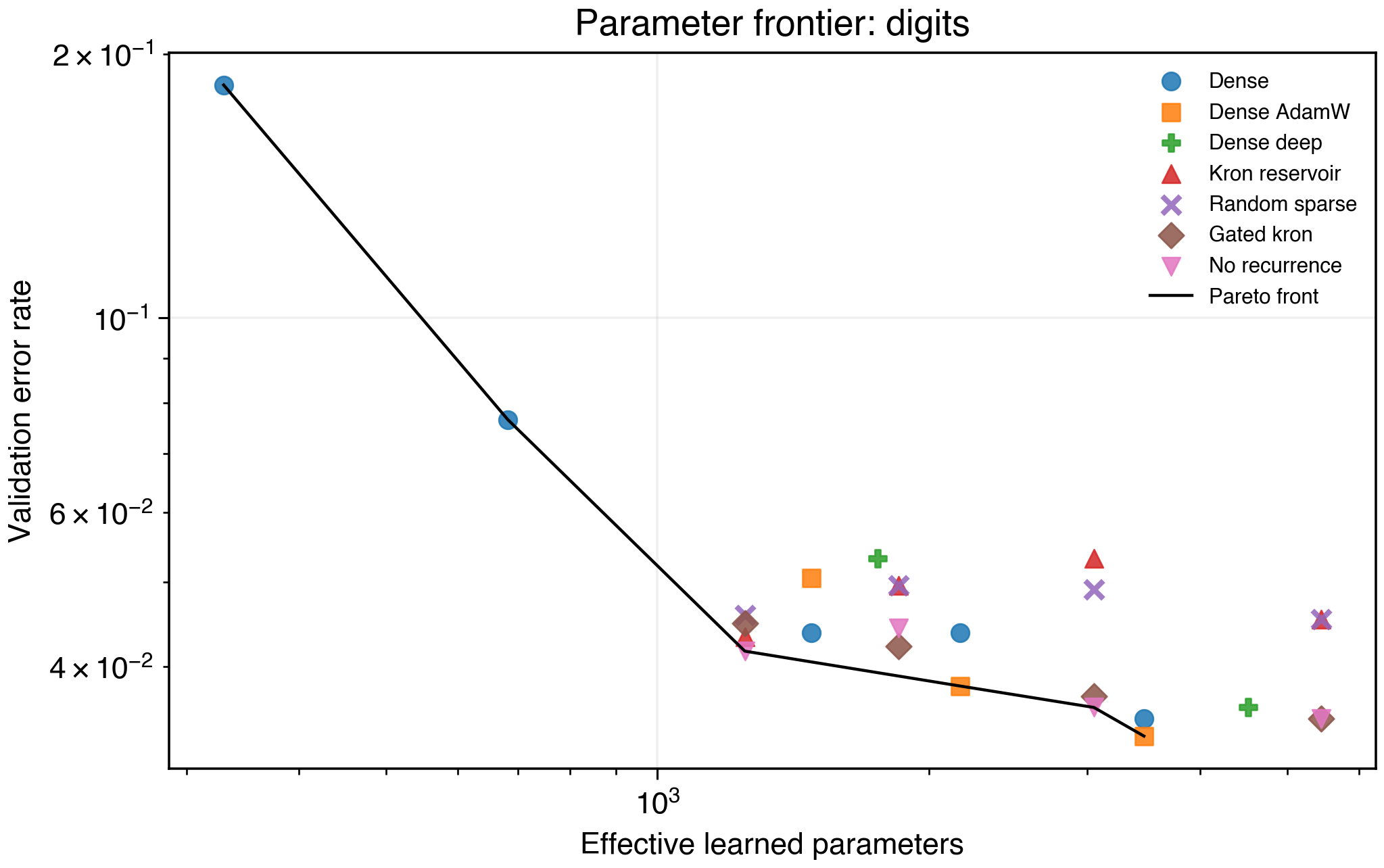
Figure 10. Digits multiclass frontier.
Digits is revealing. Dense h=8 reaches about 0.923 validation accuracy with 682 parameters. Reservoir variants can match strong accuracy, but no-recurrence expansion and dense baselines often own the frontier. On this task, the readout over expanded features matters more than the recurrent graph.
| Dataset | Main pattern |
|---|---|
| Iris | random sparse / no-recurrence expansion competitive, task is small and saturated |
| Wine | reservoirs own some low-budget frontier points |
| Digits | dense and no-recurrence expansion dominate most useful points |
| Synthetic 3-class | dense owns early frontier; no-recurrence appears at higher budget |
| Synthetic 5-class | dense and no-recurrence dominate |
Multiclass results weaken the current fractal claim. Recurrence is not automatically useful for all tabular/image-like classification. The next architecture needs a better spatial/token inductive bias before it is worth trying MNIST/Fashion-MNIST.
8. Aggregate View
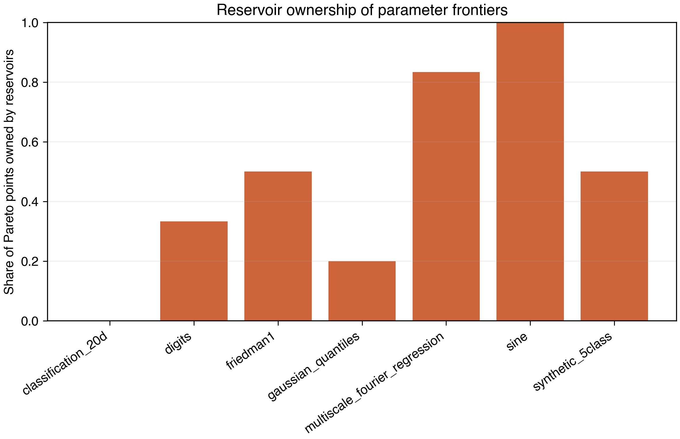
Figure 11. Fraction of each dataset’s Pareto frontier owned by reservoir/fractal families.
The pattern is consistent:
- Reservoirs are strongest at ultra-low parameter budgets.
- Smooth or low-dimensional structure favors recurrent scaffolds.
- Dense models dominate some higher-dimensional tabular and multiclass settings.
- Raw Kronecker topology is promising but not universally better than random sparse recurrence.
9. What Is Actually New Here?
The individual ingredients are known: echo state networks, sparse expansion, leaky recurrence, Kronecker structure, and looped computation. The interesting experimental object is their combination under strict parameter-frontier accounting:
\[\text{fixed multiscale recurrent scaffold} \quad + \quad \text{tiny learned input/readout} \quad + \quad \text{explicit compute-memory trade-off}.\]The current evidence supports this claim:
Small recurrent scaffold models can own the low-parameter Pareto frontier on selected synthetic tasks. The strongest current evidence is low-budget regression and saturated low-dimensional classification. The fractal/Kronecker graph is a useful candidate scaffold, but random sparse recurrence remains a serious control.
This is a good research position. It is not a final architecture yet.
10. Next Architecture Steps
The frontiers suggest how to spend the next few parameters.
Learn the initiator, not the full graph. A learned $2\times2$ or $4\times4$ initiator adds only 4-16 parameters and could adapt the graph while preserving Kronecker structure.
Add factor-level adapters. Rank-1 corrections to Kronecker factors per recurrent loop could mimic relaxed recursive transformers without learning a dense matrix.
Improve input feature maps. The classification failures suggest that the input map is too simple. A small spline/Kolmogorov-Arnold edge map before recurrence may provide better features while staying parameter efficient.
Use recurrence where topology matters. MNIST/Fashion-MNIST should wait until we test a feature extractor plus fractal reservoir head. Candidate designs:
- small CNN features followed by a fractal reservoir classifier;
- token-mixing block in an MLP-Mixer replaced by Kronecker recurrence;
- convolutional feature map flattened into a structured recurrent scaffold.
11. References
- Jaeger, H. (2001). The “Echo State” Approach to Analysing and Training Recurrent Neural Networks. German National Research Center for Information Technology GMD Technical Report, 148.
- Maass, W., Natschläger, T., & Markram, H. (2002). Real-Time Computing Without Stable States: A New Framework for Neural Computation Based on Perturbations. Neural Computation, 14(11), 2531–2560.
- Lukoševičius, M., & Jaeger, H. (2009). Reservoir Computing Approaches to Recurrent Neural Network Training. Computer Science Review, 3(3), 127–149.
- Yamashita, Y., & Tani, J. (2008). Emergence of Functional Hierarchy in a Multiple Timescale Neural Network Model: A Humanoid Robot Experiment. PLoS Computational Biology, 4(11), e1000220.
- Guerguiev, J., Lillicrap, T. P., & Richards, B. A. (2017). Towards Deep Learning with Segregated Dendrites. ELife, 6, e22901.
- Zilly, J. G., Srivastava, R. K., Koutník, J., & Schmidhuber, J. (2017). Recurrent Highway Networks. International Conference on Machine Learning, 4189–4198.
- Graves, A. (2016). Adaptive Computation Time for Recurrent Neural Networks. NIPS Workshop on Adaptive Computation and Machine Learning.
- Dehghani, M., Gouws, S., Vinyals, O., Uszkoreit, J., & Kaiser, L. (2019). Universal Transformers. International Conference on Learning Representations.
- Bai, S., Kolter, J. Z., & Koltun, V. (2019). Deep Equilibrium Models. Advances in Neural Information Processing Systems.
Let's talk!
I'm Carlo Nicolini — I am interested on the reliability of AI reasoning systems (interpretability, inference-time methods, probabilistic language programming) and on quantitative portfolio optimization (I am a maintainer of skfolio). If you're working on something in these areas and think we might collaborate, chat, discuss, I'm happy to talk about it!
The best way to reach me is on via DM on LinkedIn.