A strange echo
In a previous post on the continuous Sheffer stroke, I wrote about Andrzej Odrzywolek’s proposed eml operator (Odrzywołek, 2026). The claim is deliciously compact: the binary operation
together with the constant 1, can generate the familiar scientific-calculator basis: arithmetic, exponentials, logarithms, trigonometric functions, constants such as e, i, and pi, and then finite expressions made from them.
At first sight this sounds like a story about symbolic computation. It resembles the NAND gate: a single primitive, repeated in trees, recovers a large language of expressions. Yet the more interesting connection is with a theorem from approximation theory that has recently reappeared in machine learning: the Kolmogorov-Arnold representation theorem (Kolmogorov, 1957; Arnold, 1957).
That theorem is also the mathematical inspiration behind Kolmogorov-Arnold Networks, or KANs (Liu et al., 2025). KANs place learnable one-dimensional functions on edges and use summation at nodes. Their design turns the theorem into a neural architecture. The eml operator suggests a complementary picture: a fixed binary gate whose two input branches are already one-dimensional functions, composed repeatedly until the tree recovers elementary mathematics.
The shared pattern is simple enough to write in one line:
\[\text{one-dimensional transforms} \quad \longrightarrow \quad \text{addition} \quad \longrightarrow \quad \text{composition}.\]That is the bridge.
Kolmogorov-Arnold in one equation
The Kolmogorov-Arnold representation theorem says that every continuous multivariate function on a compact domain can be represented using sums and compositions of continuous functions of one variable. One common form is:
\[f(x_1,\ldots,x_n)= \sum_{q=1}^{2n+1} \Phi_q \left( \sum_{p=1}^{n} \phi_{q,p}(x_p) \right).\]The theorem is startling because multivariate dependence appears to have been dissolved into univariate pieces plus addition. The inner functions act separately on each coordinate. Their outputs are summed. Outer univariate functions reshape those sums. Composition ties the whole construction together.
There is a caveat. The classical theorem is existential. It guarantees continuous univariate functions, yet those functions may be irregular and hard to learn. For decades this made the result look mathematically beautiful and computationally awkward. KANs revisit the theorem with a practical engineering move: parameterize the univariate functions with splines, train them with backpropagation, and stack layers rather than insisting on the shallow original representation.
For two variables, the heart of the theorem can be compressed to the shape
\[\Phi(\phi_1(x)+\phi_2(y)).\]Once you see that shape, eml starts to look familiar.
EML as a frozen KA-style gate
The eml operator is:
Rewrite subtraction as addition:
\[\operatorname{eml}(x,y)=\exp(x)+\left(-\log(y)\right).\]Now define two univariate functions:
\[\phi_1(x)=\exp(x), \qquad \phi_2(y)=-\log(y).\]Then:
\[\operatorname{eml}(x,y)=\phi_1(x)+\phi_2(y).\]This is exactly the inner summation pattern of a two-input Kolmogorov-Arnold representation, with the important restriction that the univariate functions are fixed in advance. There is no learned spline, no family of edge functions, no adaptation to data at this level. The gate chooses two very special one-dimensional maps: exponential on the left branch and negative logarithm on the right branch.
That restriction sounds severe. Odrzywolek’s paper is surprising because repeated composition compensates for it. Instead of learning arbitrary edge functions as KANs do, EML builds binary trees:
\[S \to 1 \qquad \text{or} \qquad S \to \operatorname{eml}(S,S).\]Inputs can be added as terminals when the tree represents a function rather than a constant. The grammar is almost absurdly small. Every internal node is the same operation. Every expressive distinction lives in the tree topology and in which subtree is fed to the exponential side or to the logarithmic side.
A few identities already show the mechanism:
\[e^x=\operatorname{eml}(x,1)\]because the right branch contributes zero:
\[\log(1)=0.\]The natural logarithm can also be recovered:
\[\log(z)= \operatorname{eml} \left( 1, \operatorname{eml} \left( \operatorname{eml}(1,z), 1 \right) \right).\]The expression is less transparent than the named operation log, yet it demonstrates the deeper point. EML does not need a menu of primitives once it has a compositional route to rebuild that menu.
KANs learn the edge functions
KANs take the Kolmogorov-Arnold theorem as an architectural clue. In an MLP, edges carry scalar weights and nodes apply a fixed nonlinearity. In a KAN, edges carry learnable one-dimensional functions and nodes sum incoming values. A layer has the form:
\[x_{l+1,j} = \sum_{i=1}^{n_l} \phi_{l,j,i}(x_{l,i}).\]The functions
\[\phi_{l,j,i}\]are usually parameterized as B-splines. A full KAN is a composition of such layers:
\[\operatorname{KAN}(x) = \left( \Phi_{L-1} \circ \Phi_{L-2} \circ \cdots \circ \Phi_0 \right)x.\]This makes the network visually and mathematically interpretable. Each edge contains a one-dimensional curve that can be plotted. If a learned curve resembles a square, sine, logarithm, or rational function, the scientist has something to inspect. The KAN paper emphasizes this AI-for-science angle: the model can act as a collaborator in rediscovering symbolic structure from data (Liu et al., 2025).
So the KAN recipe is:
\[\text{learn many univariate functions, then sum and compose them}.\]The EML recipe is:
\[\text{reuse two fixed univariate functions, then sum and compose them as a tree}.\]The family resemblance is real. The difference is where expressive power is stored.
Where the expressivity lives
In a KAN, expressivity lives in the learned edge functions. The graph can be simple and regular because each edge has a flexible spline. If the target function has a compact decomposition into smooth one-dimensional pieces, a KAN can expose those pieces directly.
In an EML tree, expressivity lives in repeated composition of a single asymmetric gate. The graph itself becomes the formula. The left and right inputs are not interchangeable, since
\[\exp(x)-\log(y)\]has direction: the first argument enters through an exponential, the second through a logarithm. This chirality matters. It gives the tree enough structure to encode inverse operations, constants, arithmetic, and transcendental functions.
The contrast can be summarized as:
\[\begin{array}{c|c|c} \text{System} & \text{Univariate functions} & \text{Structure} \\ \hline \text{KAN} & \text{learned splines on edges} & \text{layered sums} \\ \text{EML} & \exp \text{ and } -\log \text{ fixed in one gate} & \text{binary trees} \\ \end{array}\]This is why the Kolmogorov-Arnold theorem feels relevant. It does not prove the EML result. Odrzywolek’s theorem is a constructive result about generating a concrete elementary-function basis from one operator and a constant. Kolmogorov-Arnold is a representation theorem for continuous multivariate functions on compact domains. The domains, goals, and proof styles differ. Still, both reveal the same structural motif: high-dimensional or apparently heterogeneous functions can be built from one-dimensional transforms, addition, and composition.
A neuro-symbolic interpretation
There is a nice neuro-symbolic way to read this.
Symbolic regression usually starts with a vocabulary:
\[\{+,-,\times,/,\exp,\log,\sin,\cos,\sqrt{\cdot},\ldots\}.\]The search problem then mixes discrete structure search with continuous parameter fitting. Which operator goes at this node? Which variables feed it? Which constants are needed? The vocabulary is powerful, yet heterogeneous.
EML replaces that vocabulary with a uniform circuit language:
\[S \to 1 \qquad \text{or} \qquad S \to \operatorname{eml}(S,S).\]This is attractive for machine learning because the architecture is regular. Every internal node is differentiable almost everywhere in the relevant numerical implementations. Odrzywolek reports experiments where shallow EML trees are optimized with Adam and can recover exact closed-form expressions from numerical data (Odrzywołek, 2026). The promise is a symbolic-regression search space with one kind of node rather than a bag of named operations.
KANs approach the same scientific desire from the other direction. They keep the graph neural and continuous, then make the learned edge curves interpretable. A trained KAN may reveal that the data want a square here, a sine there, or a low-degree interaction after summation.
So one could imagine a pipeline:
\[\text{data} \to \text{KAN} \to \text{interpretable univariate pieces} \to \text{EML or other symbolic compiler} \to \text{closed-form expression}.\]The KAN would serve as a smooth exploratory instrument. EML would serve as a compact target language for exact formulas. This is speculative, but it is a good kind of speculation: both sides already reduce the problem to univariate maps plus composition.
A small experiment: KANs as EML basin finders
The obvious weakness of EML trees is trainability. Odrzywolek’s constructive result says that the formulas exist, while the optimization problem can still be brutal. A depth-4 or depth-5 tree contains repeated exponentials and logarithms; a random initialization can easily fall into a bad numerical basin.
So I ran a small local pilot in ~/workspace/kaneml. The experiment asks a narrow question:
Can a smooth Kolmogorov-Arnold-style teacher make a tiny EML tree easier to fit?
The pipeline is:
- sample sparse noisy data from a known elementary target;
- train a small KAN-like RBF-edge teacher on those samples;
- evaluate the teacher on a dense grid inside the training domain;
- pretrain the EML tree on that dense teacher grid;
- fine-tune the same EML tree on the original sparse samples.
I also used an MLP teacher as a control. This matters because any dense teacher may act as a smoothing curriculum. If the KAN teacher helps, the correct question is whether it helps because of its Kolmogorov-Arnold structure, its smoothness, its parameter efficiency, or simply because distillation supplies more training points.
The differentiable EML node used in the pilot is a real-valued optimization surrogate:
\[\operatorname{eml}_{\mathrm{safe}}(a,b) = \exp(\operatorname{clip}(a)) - \log(\operatorname{softplus}(b)+\epsilon).\]This is not the full complex-domain EML calculus from the paper. It is a trainable real circuit that preserves the exp-minus-log asymmetry while avoiding immediate overflow and invalid logarithms.
The run was:
cd ~/workspace/kaneml
uv run python scripts/run_pilot.py --device auto --seeds 20 --quick
uv run python scripts/make_figures.py
It ran on Apple MPS over 20 seeds and three targets: a centered exponential, a shifted logarithm, and a two-variable exp-minus-log target. Each target used 48 sparse noisy training points. Success means interpolation NRMSE below 0.15 on a dense clean grid.
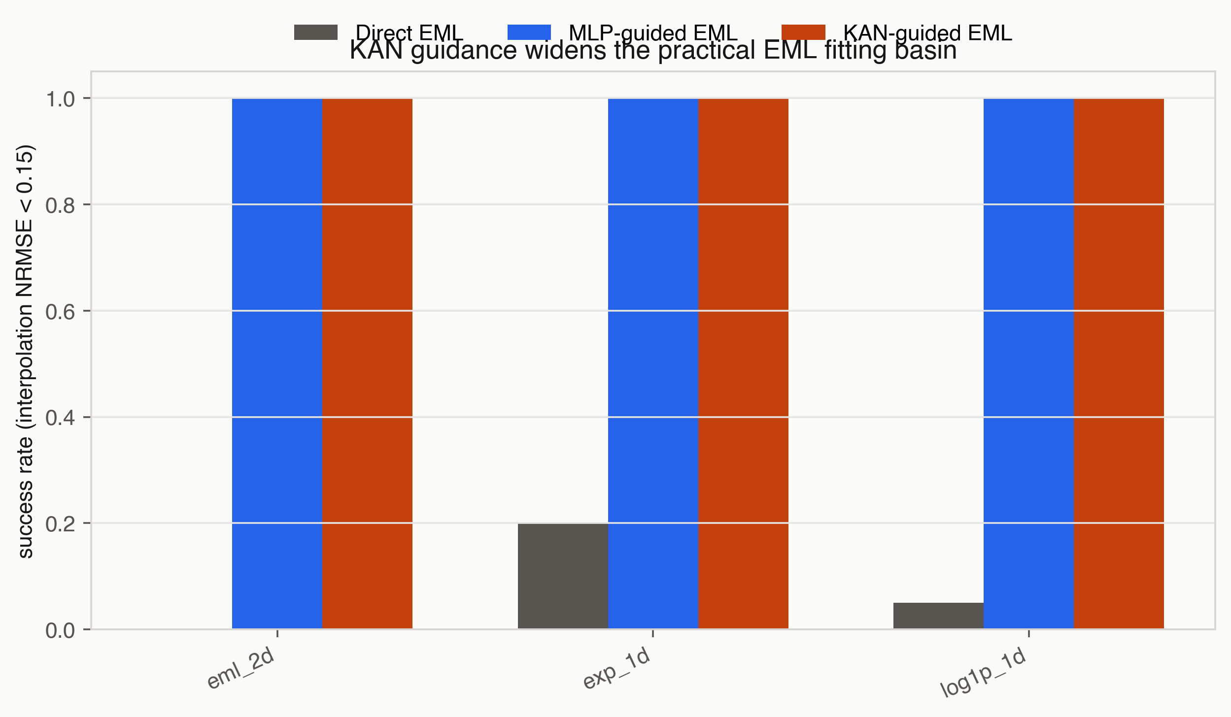
Figure 1. Teacher-guided EML trees converged reliably across the three pilot targets. Direct EML training usually stayed outside the useful basin.
| Target | Direct EML success | KAN-guided EML success | MLP-guided EML success |
|---|---|---|---|
exp_1d |
0.20 | 1.00 | 1.00 |
log1p_1d |
0.05 | 1.00 | 1.00 |
eml_2d |
0.00 | 1.00 | 1.00 |
The result is small but clean. A 32-64 parameter EML tree fails from random initialization on most seeds. The same tree succeeds after teacher-guided pretraining. On the exp target, direct EML reached mean interpolation NRMSE 0.170; KAN-guided EML reached 0.013. On the log target, direct EML reached 0.470; KAN-guided EML reached 0.022. On the two-variable EML target, direct EML reached 0.291; KAN-guided EML reached 0.042.
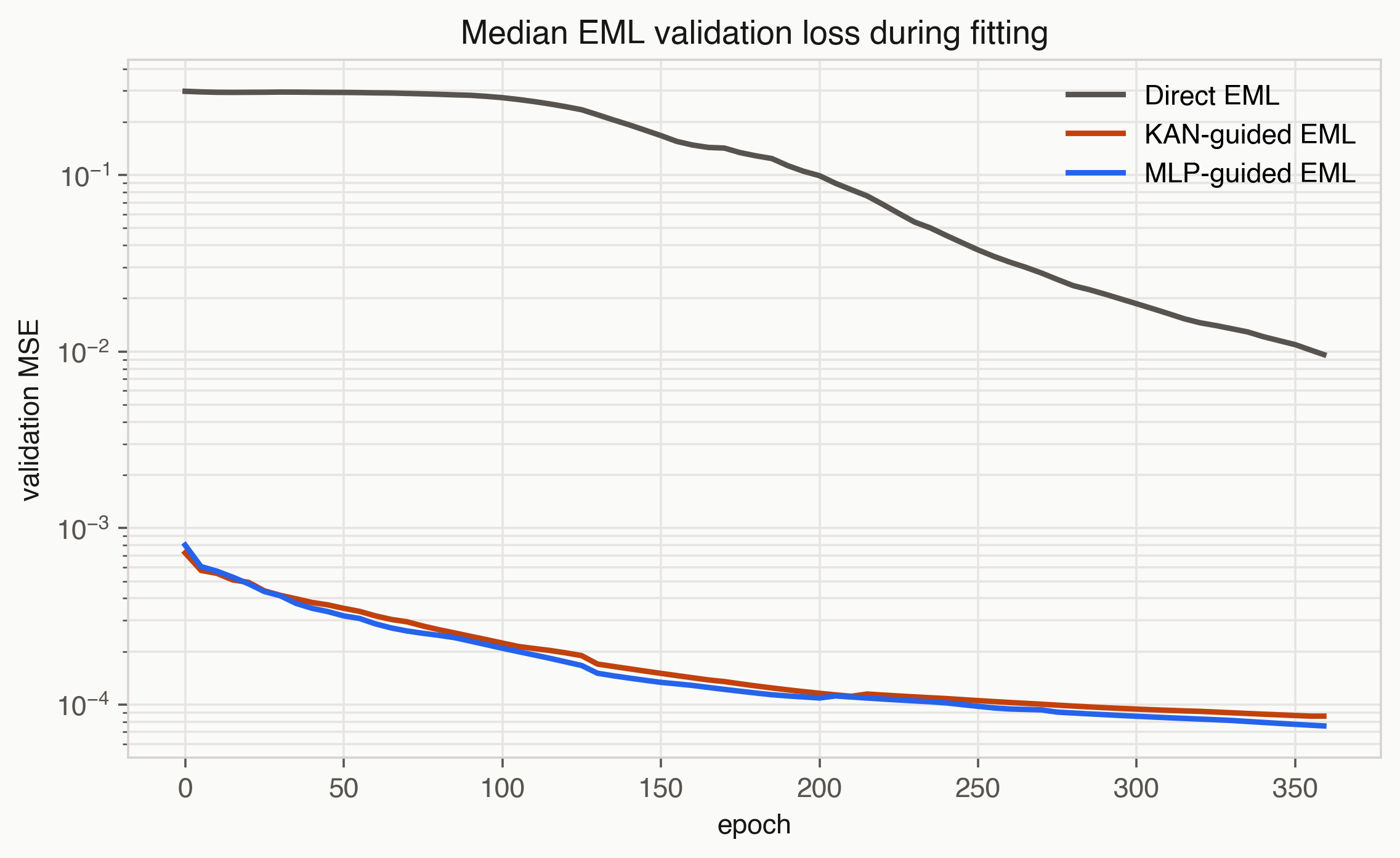
Figure 2. Median validation loss across EML routes. Teacher-guided runs enter a much better basin than direct EML.
The MLP control is important. It also helped. In fact, on the two-variable EML target the MLP teacher gave slightly lower mean extrapolation error than the KAN-lite teacher. That does not invalidate the KAN story; it sharpens it. The first robust claim is about teacher-guided basin finding for EML trees. The KAN-specific claim is more modest: a compact KAN-style teacher can provide this curriculum with far fewer parameters than the MLP teacher on these runs.
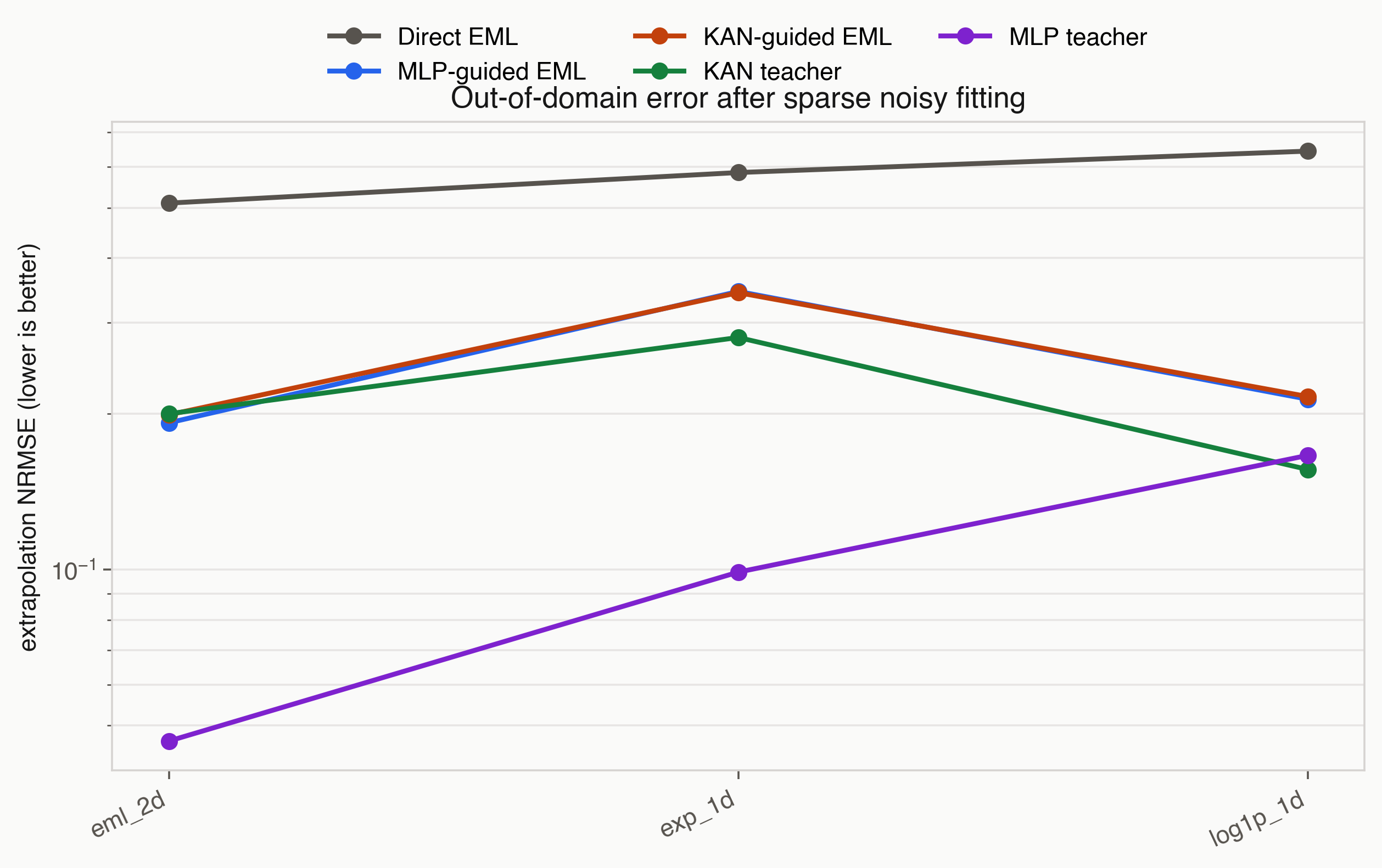
Figure 3. Extrapolation remains harder than interpolation. The guided EML trees improve sharply over direct EML, while teacher choice still matters.
The parameter counts make the compression angle visible:
| Model | Parameters on 1D targets | Parameters on eml_2d |
|---|---|---|
| KAN-lite teacher | 891 | 1323 |
| MLP teacher | 3361 | 3417 |
| EML tree | 32-64 | 40 |
The EML tree is tiny. Once a teacher gives it a useful curriculum, it can match the in-domain shape surprisingly well. Extrapolation is more mixed. For exp_1d, KAN-guided EML improves direct EML extrapolation NRMSE from 0.585 to 0.343, though the MLP teacher itself extrapolates better at 0.099. For log1p_1d, KAN-guided EML improves direct EML from 0.643 to 0.216, while the KAN teacher reaches 0.156. For eml_2d, KAN-guided EML improves direct EML from 0.510 to 0.199.
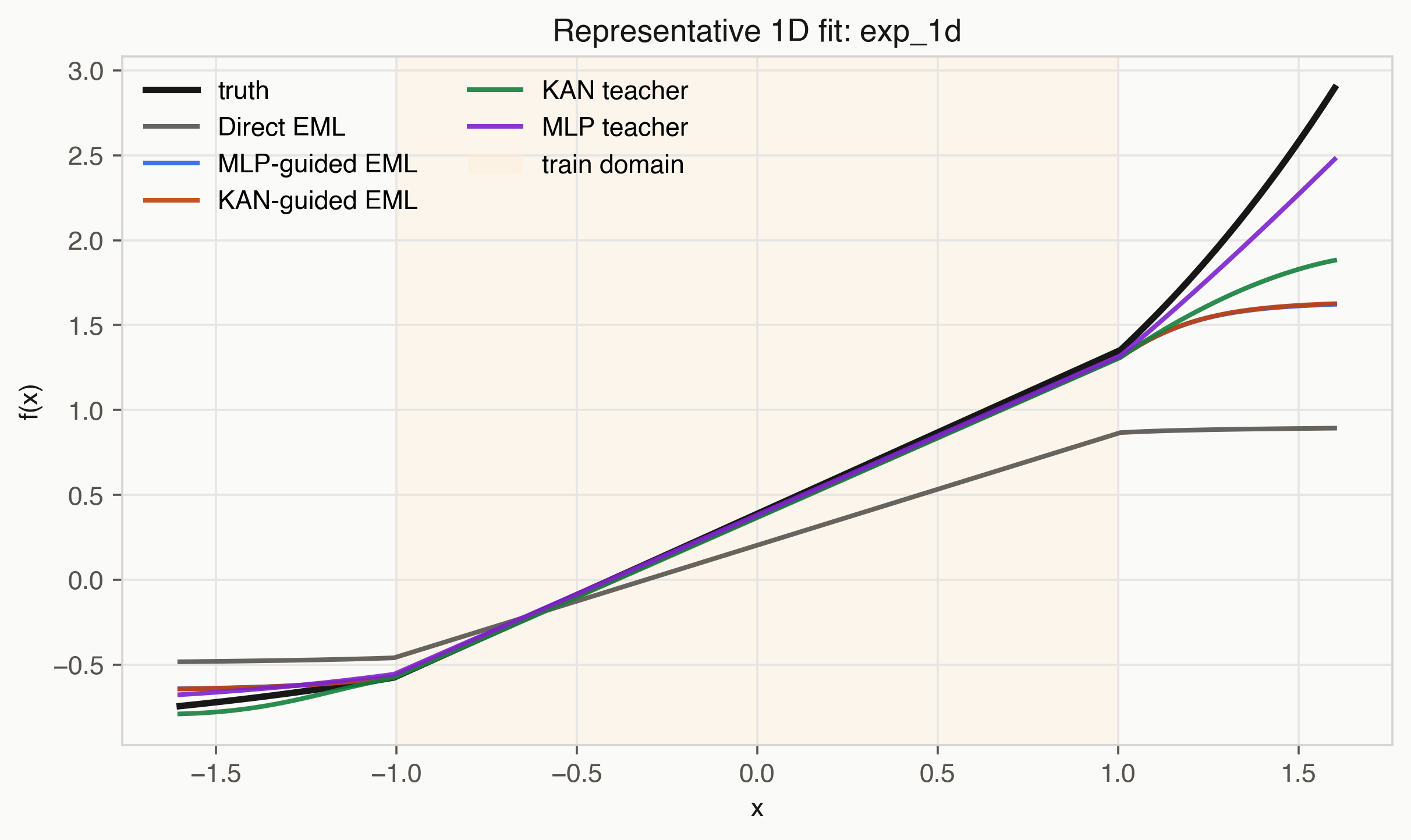
Figure 4. Representative one-dimensional fit. The shaded interval is the training domain; outside it, the teacher and EML tree can diverge.
This suggests a publishable experimental program:
- Treat KANs as smooth decomposition finders.
- Treat EML trees as a compressed homogeneous symbolic target language.
- Measure when a teacher can move EML from failed optimization to successful recovery.
- Use MLP teachers, noisy data, and extrapolation as controls.
The next experiment should separate three mechanisms: dense distillation, KAN smoothness, and KAN parameter efficiency. A stronger result would show a regime where KAN-guided EML beats MLP-guided EML at equal teacher parameter budget or equal teacher smoothness. The current pilot does not prove that yet. It gives a concrete, reproducible starting point and a better research question than the original speculation.
Why this matters
The usual story of neural networks begins with linear algebra: matrices, weights, activations, depth. The Kolmogorov-Arnold story begins with functional decomposition. It asks how much of multivariate complexity is really interaction, and how much can be moved into one-dimensional transformations followed by sums.
KANs turn that question into a trainable architecture. EML turns a related question into a symbolic basis: how small can the primitive vocabulary of elementary mathematics become?
The answer from EML is startling. A single binary gate,
\[\exp(x)-\log(y),\]plus the constant 1, appears sufficient to rebuild the scientific calculator. The answer from KANs is practical: one-dimensional functions on edges can make neural models more interpretable and sometimes more parameter efficient for scientific functions.
The shared lesson is that compositional mathematics may be much more one-dimensional than it looks. Multivariate behavior often arrives through repeated routing, summation, and reparameterization of scalar curves. KANs learn those curves. EML hard-codes two of them and lets the tree do the rest.
That is why the Kolmogorov-Arnold theorem is the right lens here. It provides the conceptual grammar in which both objects make sense.
References
- Odrzywołek, A. (2026). All elementary functions from a single operator. Arxiv:2603.21852, abs/2603.21852. https://doi.org/10.48550/arXiv.2603.21852
- Kolmogorov, A. N. (1957). On the representation of continuous functions of many variables by superposition of continuous functions of one variable and addition. Doklady Akademii Nauk SSSR, 114, 953–956.
- Arnold, V. I. (1957). On functions of three variables. Doklady Akademii Nauk SSSR, 114, 679–681.
- Liu, Z., Wang, Y., Vaidya, S., Ruehle, F., Halverson, J., Soljačić, M., Hou, T. Y., & Tegmark, M. (2025). KAN: Kolmogorov-Arnold Networks. The Thirteenth International Conference on Learning Representations. https://openreview.net/forum?id=Ozo7qJ5vZi
Let's talk!
I'm Carlo Nicolini — I am interested on the reliability of AI reasoning systems (interpretability, inference-time methods, probabilistic language programming) and on quantitative portfolio optimization (I am a maintainer of skfolio). If you're working on something in these areas and think we might collaborate, chat, discuss, I'm happy to talk about it!
The best way to reach me is on via DM on LinkedIn.