Stochastic ways to determine the laplacian spectrum
In this post I would like to describe the fashinating bridge that connects random forests, graphs, probability theory and statistical mechanics. We start from a binary undirected graph \(G=(V,E)\), and would like to find a way to sample all the random forests, i.e. the union of spanning trees that cover the whole vertex set \(V\). We denote the graph Laplacian \(\mathbf{L} = \mathbf{D} - \mathbf{A}\), where \(\mathbf{D}\) is a diagonal matrix of the node degrees, while \(\mathbf{A}\) is the adjacency matrix of the graph.
A random forests is a random combinatorial objects, like the one shown in this picture:
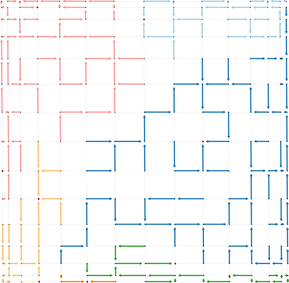
In this 15x15 grid graph, we have ran the random spanning forests algorithm as described in the following, with a value \(q=0.1\). The forests induces a partition of nodes where edges have different colours, and the root set is drawn in red.
Wilson algorithm in Python
In this section I provide a simple yet efficient implementation of the Wilson algorithm to sample random spanning. The algorithm follows this line.
- Given an undirected graph \(G=(V,E)\) with vertex set \(V\) and edge set \(E\), convert it to a directed graph, where all undirected links \((u,v)\) are replaced by two directed links \((u,v)\) and \((v,u)\). If the graph is binary, set edge weights to 1.
- Add a node called root to the graph \(G\).
- Connect all nodes with directed edges to the root node with weight \(q\). Do not connect \(r\) to all other nodes in the other direction.
- Sample a random spanning tree starting from a random node (not \(r\)).
- Eliminate the root node \(r\) together with all its connections.
The point 4 has to be elaborated a bit, but the pseudocode is made clear in the two methods Wilson.sample() and Wilson.random_successor(), and is very similar to the original pseudocode described in the Wilson paper [1]. I will not describe it here. I only specify that in order to sample a random Markov walk with weighted edges, one has to find a way to sample from a non-uniform distribution. This is done in the numpy function np.random.choice(nei, p = weight) with the weights computed as the sum of incident edge weights to the node.
Moreover, the role of \(q\) is crucial. Large values of \(q\) and the result is a degenerate forests made of singleton nodes. Small values of \(q\) and the random forest is a random spanning tree. This gives the idea that this random process has a lot to tell about the topology of the graph, but most surprisingly it tells a lot about the Laplacian eigenvalues \(\lambda_i\).
Importantly, one of the main results of this sampling algorithm is that the set of roots are well separated a mathematical notion pretty complicated to explain (see references below), but that corresponds to the intuition that the roots are never too far or too close, and that they locally represent the link density of graph.
The directed graph induced after the remotion of the root node \(r\) is a random spanning forests, i.e. a random variable \(\Phi_q\) sampled from the following probability distribution
\[\mathbb{P}(\Phi_q = \phi) = \frac{w(\phi) q^{|\mathcal{R}(q)|}}{Z(q)}\]where \(\mathcal{R}(\phi)\) is the set of roots of the trees in the forest. The root vertices are such that, given any other vertex in the tree, following the directed edges in the tree you always reach the root. The quantity \(Z(q)\) is a partition function and sums the numerator over all possible random spanning forests (denoted by the set \(\mathcal{F}\))
\[Z(q) = \sum \limits_{\phi \in \mathcal{F}} w(\phi)q^{|\mathcal{R}(q)|}\]A variant of the Markov chain tree theorem applies here, telling us that the partition function is nothing else than the characteristic polynomial of the negative Laplacian \(-\mathbf{L}\).
\[Z(q) = \det\left(q \mathbf{I} + \mathbf{L} \right) = \prod \limits_{i=1}^n (q + \lambda_i)\]It’s great to see that the Wilson algorithm is the correct way to sample from this highly complicated probability law. Interestingly, we can use the Wilson algorithm to study spectral properties of the network Laplacian. With the partition function in our hand, we can take the logarithm and see that we can generate the moments of the distribution of the random variable \(|\mathcal{R}(\phi)|\).
In particular we can form a stochastic unbiased estimator of
\[q\mathrm{Tr}\left \lbrack \left( q\mathbf{I} + \mathbf{L} \right)^{-1} \right \rbrack\]by looking at the average number of roots, given \(q\):
\[\mathbb{E}[|\mathcal{R}_q(\phi)|] = q\mathrm{Tr}\left \lbrack \left( q\mathbf{I} + \mathbf{L} \right)^{-1} \right \rbrack\]For example, for the ring of cliques graph shown in the picture below and only 2 random samples we have a very good approximation of \(q\mathrm{Tr}\left \lbrack \left( q\mathbf{I} + \mathbf{L} \right)^{-1} \right \rbrack\) by using the average number of roots.
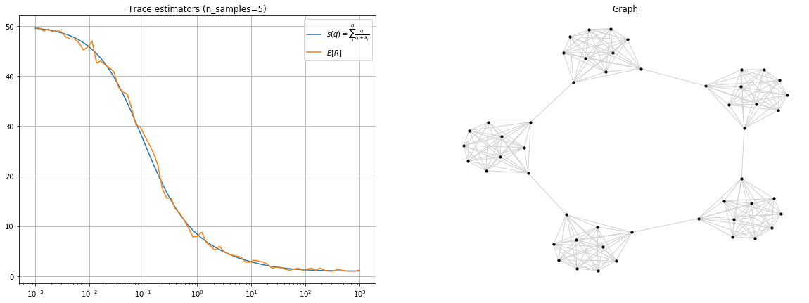
Trace estimator via Wilson algorithm on a ring of cliques.</figcaption> </figure>
There are also interesting links with statistal mechanics here. If we use the properties of the matrix determinant, we know that it is equivalent to the product of the eigenvalues of the matrix. Hence in our case we have
\[\chi(q) = \det( q\mathbf{I} + \mathbf{L}) = \prod \limits_{i=1}^n (q + \lambda_i)\]but manipulating this last expression a bit in terms of matrix logarithms we find
\[\chi(q) = e^{\mathrm{Tr}\lbrack \log(q\mathbf{I} + \mathbf{L}) \rbrack}\]Taking the logarithm of the partition function we find
\[\log \chi(q) = \mathrm{Tr}\lbrack \log(q\mathbf{I} + \mathbf{L}) \rbrack\]With some other simple manipulations and setting \(q=\beta^{-1}\) we obtain:
\[\log \chi(\beta^{-1}) = \mathrm{Tr}\lbrack \log(I+\beta \mathbf{L}) -n\log \beta \rbrack\]This expression starts reminding us about the Boltzmann partition function \(\chi(\beta)=\mathrm{Tr}\left \lbrack e^{-\beta \mathbf{L}} \right\rbrack\). Indeed if we Taylor expand both of them in the limit \(\beta \to 0\), equivalent to large \(q\), hence many small trees in the forest, we can see that:
\[Z \approx n - \log \chi(\beta^{-1}) + n\log \beta + r(\beta)\]The residual term \(r(\beta)\) is written as
\[r(\beta) = \sum_{k=3}^{\infty}\left(\frac{(-1)^k}{k!} - \frac{(-1)^{k+1}}{k} \right) \beta^k \mathrm{Tr}\lbrack \mathbf{L}^k \rbrack\]This approximation tells us that the Boltzmann partition function in the spectral entropies framework is describing the combinatorial statistics of random spanning forests in the graph, at least in the limit of many small trees. It’s indeed very good, until the limit \(\beta = (\lambda_{max})^{-1}\) which is the limit in which we can Taylor expand the Mercator series of the logarithm.
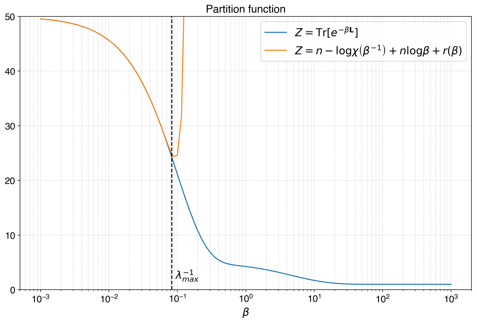
In this picture the limit of the approximation is exactly \(1/\lambda_{max}\). For values of \(\beta\) lower than this threshold, the approximation is incredibly good, and it definely links the partition function to the combinatorics of random spanning forests as from the Wilson algorithm.</figcaption> </figure>
In this picture the limit of the approximation is exactly \(1/\lambda_{max}\). For values of \(\beta\) lower than this threshold, the approximation is incredibly good, and it definitely links the partition function to the combinatorics of random spanning forests as from the Wilson algorithm.
From approximation to exact relation: inverse Laplace transform
Incredible as it was to find this approximation, we don’t have to stop there. As I recently detailed in a new preprint (Nicolini, 2025), there is an exact analytic relation bridging the expected number of roots \(s(q)\) in random spanning forests to the heat-trace partition function \(Z(\beta)\).
Starting from the resolvent trace identity:
\[\frac{s(q)}{q} = \mathrm{Tr}\left \lbrack (q\mathbf{I} + \mathbf{L})^{-1} \right \rbrack = \sum_{i=1}^n \frac{1}{q+\lambda_i}\]We can use the elementary integral identity \(\frac{1}{1+a} = \int_0^\infty e^{-(1+a)t} dt\) to replace the denominator. With some algebra, setting \(a=\lambda_i/q\) and \(t=q\beta\), we find that:
\[\frac{s(q)}{q} = \int_0^\infty e^{-q\beta} \left( \sum_{i=1}^n e^{-\beta\lambda_i} \right) d\beta = \int_0^\infty e^{-q\beta} Z(\beta) d\beta = \mathcal{L}_\beta[Z](q)\]This key result establishes that the resolvent trace \(s(q)/q\) is exactly the Laplace transform in \(q\) of the spectral entropy partition function \(Z(\beta)\).
Why is this important? It means that we can recover global thermodynamic observables such as the partition function, energy, and Von Neumann entropy without performing a costly full Laplacian eigendecomposition. By using the Wilson algorithm to sample random forests, we obtain unbiased Monte Carlo estimators for \(s(q)/q\). We can then invert the Laplace transform to reconstruct \(Z(\beta)\) accurately across all temperature scales \(\beta\).
Network Observables from Forest Statistics
Beyond global thermodynamic observables, this forest representation naturally suggests local descriptors attached to nodes and edges. For a given realization of the random forest \(\Phi_q\), we define the node-level indicator \(X_v(q) = \mathbf{1}\\{v \in \mathcal{R}(\Phi_q)\\}\). Its expectation gives the local occupation probability for a vertex \(v\):
\[\pi_v(q) = \mathbb{P}(v \in \mathcal{R}(\Phi_q)) = q[(q\mathbf{I} + \mathbf{L})^{-1}]_{vv}\]Summing this probability over all vertices recovers the expected root count \(s(q)\). Expanding in the spectral basis, we find:
\[\pi_v(q) = q \sum_{i=1}^n \frac{u_{iv}^2}{q+\lambda_i}\]where \(u_i\) are the orthonormal eigenvectors of \(\mathbf{L}\). The root probability of a node is thus a superposition of spectral modes, modulated by the local eigenvector weights \(u_{iv}^2\).
A similar construction applies to edges. For an undirected edge \(e = \\{u,v\\}\) with weight \(w_{uv}\), we measure how likely it is to participate in the forest:
\[\theta_e(q) = \mathbb{P}(e \in \Phi_q) = w_{uv} \left[ (q\mathbf{I} + \mathbf{L})^{-1}_{uu} + (q\mathbf{I} + \mathbf{L})^{-1}_{vv} - 2(q\mathbf{I} + \mathbf{L})^{-1}_{uv} \right]\]This coincides with the edge weight multiplied by a \(q\)-dependent effective resistance between \(u\) and \(v\). In the spectral basis, it becomes:
\[\theta_{\{i,j\}}(q) = w_{ij} \sum_{k=1}^n \frac{(u_{ki} - u_{kj})^2}{q+\lambda_k}\]Both \(\pi_v(q)\) and \(\theta_e(q)\) constitute local thermodynamic fingerprints of the graph that can be directly estimated via Wilson sampling without eigendecomposition.
Numerical Inverse Laplace Transform via Stieltjes Spectral Density
The classical Gaver-Stehfest algorithm for inverse Laplace transforms is notoriously sensitive to numerical noise, which is problematic when using Monte Carlo estimates for \(s(q)/q\). A more robust approach relies on a Stieltjes spectral-density regularization.
We can define the spectral density as \(p(\lambda) = \frac{1}{n} \sum_{i=1}^n \delta(\lambda - \lambda_i)\) such that \(\int_0^\infty p(\lambda) d\lambda = 1\). The resolvent trace can then be rewritten as a Stieltjes transform:
\[g(q) = \frac{s(q)}{q} = \sum_{i=1}^n \frac{1}{q+\lambda_i} = n \int_0^\infty \frac{p(\lambda)}{q+\lambda} d\lambda\]To invert this, we can approximate \(p(\lambda)\) on a grid of spectral abscissae \(\\{\lambda\_k\\}\_{k=1}^{N\_{\lambda}}\) with log-spaced bin widths \(\Delta\lambda_k\), representing the density as piecewise constant coefficients \(p_k\). By gathering our Monte Carlo estimates \(g(q_j)\) from Wilson sampling into a data vector \(\hat{\mathbf{g}}\) with inverse-variance weight matrix \(\mathbf{W}\), the forward model becomes \(\hat{\mathbf{g}} \approx \mathbf{A}\mathbf{p} + \boldsymbol{\varepsilon}\).
The reconstruction of the spectral density \(p(\lambda)\) is cast as a nonnegative Tikhonov minimization problem:
\[\mathbf{p}^\star = \arg\min_{\mathbf{p} \ge 0} \left\| \mathbf{W}^{1/2} (\mathbf{A}\mathbf{p} - \hat{\mathbf{g}}) \right\|_2^2 + \gamma_{\mathrm{mass}} \left( \sum_{k=1}^{N_\lambda} \Delta\lambda_k p_k - 1 \right)^2 + \tau_{\mathrm{smooth}} \| \mathbf{D}\mathbf{p} \|_2^2\]Here, the first term minimizes the weighted least-squares error against the Monte Carlo sampling, the second term enforces the spectral density normalization constraint, and the third term (using the second-difference matrix \(\mathbf{D}\)) suppresses spurious noise-induced oscillations.
Finally, having recovered a robust and smooth approximation of the spectral density \(\mathbf{p}^\star\), the partition function is stably reconstructed by forward quadrature:
\[Z(\beta) \approx n \sum_{k=1}^{N_\lambda} p_k^\star e^{-\beta\lambda_k} \Delta\lambda_k\]This operational framework provides a unified bridge between the combinatorics of spanning forests and the heat-kernel thermodynamics of complex networks, capable of handling sampling noise and bypassing exact eigendecompositions. You can read the full details, derivations, and numerical experiments in the paper: Spectral Entropy via Random Spanning Forests (Nicolini, 2025).
Code
Here is the code needed to generate all these figures. It’s written in Python and it explains the details of the Wilson algorithm in the function sample.
#!/usr/bin/env python3
"""
Wilson's algorithm for unweighted STs.
"""

import numpy as np
import networkx as nx
import matplotlib.pyplot as plt
import random
import matplotlib

class Wilson:

    def __init__(self, G, q):
        self.G = G
        self.H = nx.DiGraph()
        self.nv = G.number_of_nodes()
        self.q = q
        self.L = nx.laplacian_matrix(self.G).toarray()

        # set edge attribute weight with weight 1
        self.H.add_weighted_edges_from([(u,v,1.0) for u,v in G.edges()])
        self.H.add_weighted_edges_from([(v,u,1.0) for u,v in G.edges()])

        # add links from all nodes in the original graph to the root with weight q
        self.root = self.nv
        self.H.add_weighted_edges_from([(u,self.root, q) for u in G.nodes()])

    # Choose an edge from v's adjacency list (randomly)
    def random_successor(self, v):
        nei = list(self.H.neighbors(v))
        weight = np.array([ self.H.get_edge_data(v,u)['weight'] for u in nei], dtype=float)
        weight /= weight.sum()
        return np.random.choice(nei, p = weight)

    def sample(self):
        intree = [False] * self.H.number_of_nodes()
        successor = {}
        # put the additional node
        F = nx.DiGraph()
        self.roots = set()
        root = self.nv
        intree[root] = True
        successor[root] = None

        from random import shuffle
        l = [root] + list(range(self.nv))
        shuffle(l) # not necessary but nice, since the results do not depend on the order
        for i in l:
            u = i
            while not intree[u]:
                successor[u] = self.random_successor(u)
                if successor[u] == self.nv: # if the last node of the trajectory is ∆ add it to the roots
                    self.roots.add(u)
                u = successor[u]
            u = i # come back to the node it started from
            # remove self-loops
            while not intree[u]:
                intree[u] = True
                #if u in successor:
                u = successor[u]

        # Creates the random forest
        for i in range(self.nv):
            if i in successor.keys():
                neighbor = successor[i]
                if neighbor is not None:
                    F.add_edge(i,neighbor)

        if self.nv in self.roots:
            self.roots.remove(self.root)
        # remove the root node, together with all its links
        F.remove_node(self.root)
        # save the leaves
        # self.leaves = [n for n in F.nodes() if F.degree(n)==1]
        return F, list(self.roots)

    def s(self):
        lambdai = np.linalg.eigvalsh(self.L)
        return (self.q/(self.q + lambdai)).sum()

def draw_sampling(G, T, root_nodes=None, **kwargs):
    ax = kwargs.get('ax',None)
    cmap = kwargs.get('cmap', matplotlib.cm.get_cmap('Set3'))
    T = nx.DiGraph(T)
    n_trees = nx.number_weakly_connected_components(T)
    pos = nx.spectral_layout(G)
    if root_nodes is not None:
        nx.draw_networkx_nodes(G, pos=pos, nodelist=root_nodes, node_color='r',node_size=25,linew_width=1,ax=ax)
        #nx.draw_networkx_labels(G, pos=pos, labels={i: i for i in range(G.number_of_nodes())})
    nx.draw_networkx_nodes(G, pos=pos, node_color='k', node_size=3, lines_width=0.1,ax=ax)
    nx.draw_networkx_edges(G, pos, edge_style='dashed', alpha=0.1, edge_color='k', edge_width=0.01, ax=ax)

    for i, t in enumerate(nx.weakly_connected_component_subgraphs(T)):
        e = nx.number_of_edges(t)
        #print('|V|=%d |E|=%d' % (t.number_of_nodes(),t.number_of_edges()))
        nx.draw_networkx_edges(t, pos, width=4, edge_cmap=cmap, edge_color=[cmap(float(i)/n_trees)]*e ,ax=ax, arrows=True)
        #nx.draw_networkx_edges(t, pos, width=1, edge_color='k', arrows=True,ax=ax)
    plt.axis('off')

def trace_estimator(G):
    reps = 1
    beta_range = np.logspace(-2, 2, 100)
    L = nx.laplacian_matrix(G).toarray()
    plt.semilogx(beta_range, [np.mean([len(Wilson(G,1/beta).sample()[1]) for _ in range(reps)]) for beta in beta_range], label='E[|R|]')
    plt.semilogx(beta_range, [Wilson(G,q=1/beta).s() for beta in beta_range], label='q Tr[(qI+L)^{-1}]' )
    plt.legend()
    plt.grid(which='both')
    plt.show()

def sampling_example(G):
    q = 0.1
    W = Wilson(G, q=q)
    F,roots = W.sample()
    draw_sampling(G, F, roots)
    plt.show()

if __name__=='__main__':
    G = nx.grid_2d_graph(15, 15, periodic=False)
    G = nx.from_numpy_array(nx.to_numpy_array(G))

    trace_estimator(G)
    sampling_example(G)
References
This post is just a very small part of a large literature on random spanning trees and forests in graph, and their link with random walks on graphs. Some references are these. In particular my implementation of the Wilson algorithm is based on reference [1].
- Bruce Wilson: Generating random spanning trees more quickly than the cover time.
- Propp and Wilson: How to Get a Perfectly Random Sample from a Generic Markov Chain and Generate a Random Spanning Tree of a Directed Graph. Journal of Algorithms. 10.1006/jagm.1997.0917
- Luca Avena, Alexandre Gaudilliere: Random spanning forests, Markov matrix spectra and well distributed points. Arxiv 1310.1723
- Luca Avena, et al. Random Forests and Networks Analysis. J. Stat. Phys. (2018)
- Lyons, Russell and Peres, Yuval: Probability on trees and networks. Cambridge Univ.Press (2017)
References
- Nicolini, C. (2025). Spectral Entropy via Random Spanning Forests. Arxiv:2512.13318.
Let's talk!
I'm Carlo Nicolini — I am interested on the reliability of AI reasoning systems (interpretability, inference-time methods, probabilistic language programming) and on quantitative portfolio optimization (I am a maintainer of skfolio). If you're working on something in these areas and think we might collaborate, chat, discuss, I'm happy to talk about it!
The best way to reach me is on via DM on LinkedIn.