In this post I would like to introduce to the nilearn user, a modified set of functions based on the nilearn.surface module, that are of great help in making beautiful surface colored pictures of brain, like the one in this figure:

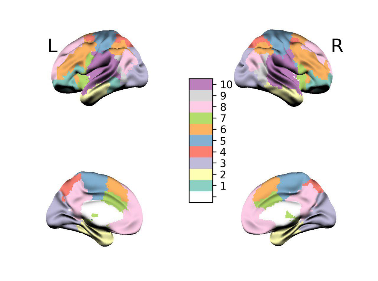
Image of the results of a Modularity analysis of brain functional connectivity of resting state healthy patients

For this picture, I took inspiration from the wonderful toolbox BrainetViewer by Mingrui Xia. Unfortunately the toolbox is only available in Matlab, and similar results were difficult to obtain with standard Python toolboxes.

The mesh shown in this example is obtained from BrainetViewer. It is a .nv file contained in the SurfData folder in BrainetViewer, the file is BrainMesh_ICBM152_smoothed.nv. The mesh file that contains only vertices and indices of the triangles (with indices starting from 1). In the following parts, I will detail step by step how to make such a beatiful plots, how to avoid typical errors and finally the code that does this wonderful picture.

Why this post?

I have found that Python still lacks a decent way to integrate beatiful visualization of brain templates with the results of network community detection. That’s what is typically needed in the pipeline of analysis of connectomic data, as well as in the graph-theoretical treatment of brain data.

Most important, working with seaborn and a number of other libraries based on matplotlib, I needed to be able to put my results into matplotlib axes, as subplots. There are a number of libraries out there which can plot parcellized areas over a brain surface, but I did not have the degree of control over the colormaps, the brain surface and a number of other minor quirks. For this reason I preferred to make my own functions for this task. I like home-made implementation of the stuff that I base my research on.

To be clear, I had a pandas dataframe, where a column contain a numpy array with the node label assignments, and based on some other columns I wanted to do facetings to quickly visualize the effects of two variables, store in columns var1 and var2 on the parcellation of the brain.

What do I need to make this beatiful plots?

Ingredients:

A working Python3 installation, with the pip3 package installed. Doing this in Linux distribution is highly suggested.
A nifti template. You can download one here.
A vector of integers with the same length as the total number of parcels in the nifti template.
A mesh of the brain surface to render. Here I use
Some time to read and understand.

All the ingredients of this recipe are baked and ready to be used in a simple Python3 package that I developed for the laziest people out there. The package is called brainroisurf and is available at my github page.

Link to the code

https://github.com/carlonicolini/brainroisurf

The package already contains a number of example data, templates and surfaces files. Just follow the instructions at the README and you’ll be ready.

In the next lines, I will better detail the inner workings of this package.

Why is this visualization useful?

We often work with community detection methods applied to brain connectivity. In the paradigm of the study of functional connectivity with complex network methods, we typically implement the following recipe:

We get a Nifti template, that assigns each voxel an integer number. Examples of these templates are the AAL120, or the Harvard-Oxford template, or the Destrieux atlas. A number of templates is available in the literature. In my pipeline I often use a template from Craddock et. al with 638 areas. This template is available here.
From the nifti template, one creates a network (i.e. an adjacency matrix that we indicate as ) based on the number of areas defined by the template. This means we have a network with 638 nodes. Depending on the dataset we are going to analyze then we define the strength of the links between the template-defined nodes as the correlation between the averaged time series of all voxels defined in the same parcel.
Once we have a graph, we compute some metrics on it. We are interested in the communities of the network. Communities are loosely defined as groups of nodes in a network that are tightly bound together, and loosely connected to each other. Algorithms like the Louvain method for optimizing the modularity return as result a vector of memberships of each node. In this case we will have a vector of 638 integers, where at i-th element of the vector m, i.e. m[i], we have the index of the community that the node belongs to.
While we more or less have a way to visualize the nifti template (using nilearn.plotting.plot_roi method), we instead want to change the content of the voxels based on the content of the vector m[i], that we use to relabel the areas of the template. Something that nilearn is able to do, but with some small problems as in Figure 2.
We iterate over the range $[0,638]$ with the variable i and assign the voxels in the template with value i, the value of the corresponding membership m[i].
We then must project on the surface of the brain, the values contained in the volume. There are a number of problems in doing this. When computing the color of a vertex of the mesh, we must decide which value of the voxel we should keep. To make beatiful surface renderings, we choose to use the value of the majority of the voxels close to the surface.
We also need to use a decent colormap. A good colormap must assign integer number to discrete colors, possibly maximally perceptually different, and with the gray color assigned to the 0, which in the nifti is the number assigned to empty space.

This visualization has a number of problems. You cannot use this colormap for discrete data, and with just 7 classes the choice of colors is not the best one can use.

The problems we address

It looks like our brain parcellated surface can be plotted with a smart usage of the nilearn.surface.plot_surf_roi method.

Unfortunately, the result is horrible and is shown in the following figure.

We are limited to the default brain surface. Even if we could in theory use other surfaces, by providing vertices and faces of a mesh, we miss a decent lightning model to shade the surface. Moreover there is a not very nice interpolation of colors between different areas, which we don’t want, being our data discrete, and the general color map is not adequate to our purpose.

Can we make something like Figure 2 but in 3D and visualized as a surface?

Loading the mesh and computing normals

As we want to be able to work with any surface mesh of the brain we want, we must load the mesh in Python. To load the .nv files, I provide a set of functions that load the data, compute the normals of the faces and average each normal face over the vertices.

def normalize_v3(arr):
    """ Normalize a numpy array of 3 component vectors shape=(n,3) """
    lens = np.sqrt(arr[:, 0]**2 + arr[:, 1]**2 + arr[:, 2]**2)
    # hack
    lens[lens == 0.0] = 1.0
    arr[:, 0] /= lens
    arr[:, 1] /= lens
    arr[:, 2] /= lens
    return arr

def compute_normals(vertices, triangles):
    # Create a zeroed array with the same type and shape as our vertices i.e., per vertex normal
    norm = np.zeros(vertices.shape, dtype=vertices.dtype)
    # Create an indexed view into the vertex array using the array of three indices for triangles
    tris = vertices[triangles]
    # Calculate the normal for all the triangles, by taking the cross product of the vectors v1-v0, and v2-v0 in each triangle
    n = np.cross(tris[::, 1] - tris[::, 0], tris[::, 2] - tris[::, 0])
    # n is now an array of normals per triangle. The length of each normal is dependent the vertices,
    # we need to normalize these, so that our next step weights each normal equally.
    normalize_v3(n)
    # now we have a normalized array of normals, one per triangle, i.e., per triangle normals.
    # But instead of one per triangle (i.e., flat shading), we add to each vertex in that triangle,
    # the triangles' normal. Multiple triangles would then contribute to every vertex, so we need to normalize again afterwards.
    # The cool part, we can actually add the normals through an indexed view of our (zeroed) per vertex normal array
    norm[triangles[:, 0]] += n
    norm[triangles[:, 1]] += n
    norm[triangles[:, 2]] += n
    normalize_v3(norm)
    return norm

def load_nv(filename):
    '''
    Load files in the .nv format as the Surf data in the BrainetViewer
    First line is a comment and is skipped
    '''
    import itertools
    num_vertices = int(open(filename).readlines()[1])
    num_faces = int(open(filename).readlines()[2+num_vertices])
    XYZ, faces = None, None
    with open(filename) as f_input:
        XYZ = np.loadtxt(itertools.islice(f_input, 0, num_vertices+2),
                         delimiter=' ', skiprows=2, dtype=np.float32)
    with open(filename) as f_input:
        faces = np.loadtxt(itertools.islice(f_input, num_vertices+3,
                                            num_vertices+num_faces+3),
                            delimiter=' ', skiprows=0, dtype=np.int32)
    return XYZ, faces - 1

Definining a decent colormap

We need a discrete colormap. We like to count color classes with numbers from 1 to C and reserve the 0 for the unmapped. Here we create a colormap for a large number of classes, with maximally perceptually different colors, to be used by colorblind people and whose grayscale conversion still conveys different tones. A colormap like this is implemented in the wonderful color library colorbrewer2. Luckily Python has a module named brewer2mpl that allows to convert the wonderful colorbrewer maps into a matplotlib.color.LinearSegmentedColormap. With the function here, one only needs to select how many classes and the name of the colormap to produce a already usable colormap. Moreover, if the option add_gray is set to True, a white color is insterted for the class 0.

def create_mpl_integer_cmap(name, num_classes, add_gray=True):
    import brewer2mpl
    from matplotlib import colors
    bmap = brewer2mpl.get_map(name, 'qualitative', num_classes)
    from copy import copy
    cols = copy(bmap.mpl_colors)
    if add_gray:
        cols.insert(0,[0,0,0,0]) # add black for the unmapped areas
    cmap = colors.LinearSegmentedColormap.from_list(name, cols)
    return cmap

The colormap of the first figure in this post is Set3 with 10 classes and the white mapped to 0. We now want to compute the colors for a vector memb that contains the membership of our nodes in the graph. The vector memb has values between 0 and 9. With the following code you can taste the effect of a correct colormap over discrete data:

from mpl_toolkits.mplot3d import Axes3D
import matplotlib.pyplot as plt
import numpy as np

from matplotlib import cm
nx = 9
memb = np.linspace(0, nx, nx)
cmap = create_mpl_integer_cmap('Set3', int(np.max(memb)))
fig = plt.figure()
#plt.imshow(memb.reshape([1, nx]), cmap=cmap, interpolation='none')
#plt.xticks(dict(zip(range(0,nx),memb)))
plt.axis('off')
m = cm.ScalarMappable(cmap=cmap)
C = int(np.max(memb))
m.set_array(memb)
values = np.linspace(np.min(memb),np.max(memb),np.max(memb))
cbar = fig.colorbar(m, shrink=0.75, aspect=5, boundaries = range(0,C+2), values = range(0, C + 2))
cbar.set_ticks( np.array(range(0, C + 1)) + 0.5 )
cbar.set_ticklabels( ['unmapped'] + list(range(1, C + 1)) ) # height of tick labels

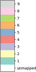
*A colorbar with 9 unique discrete values, and the 0 left as unmapped.

Mapping the membership vector to mesh vertices

You need to change the value in the volume using the values from the membership vector. As every voxel belongs to one of the $C$ classes in the membership vector, the simplest way to do that is to iterate over the parcels, find the voxels within the parcel and assign those voxels the block specified by the membership vector.

Ain’t easy? Just run a for loop over the membership vector. The smaller the number of parcels and the smaller the template, the faster the loop. There is still room for improvement here, I believe. We do the thing in two passages. We first collect the indices (i,j,k) of the voxels belonging to parcel membership[parcel] and then we imbue those voxel with the right value. This is done to avoid overwriting the same array twice.

Finally we apply the customized surface.vol_to_surf function, specifying as the interpolation nearest (for nearest neighbor sampling of mesh vertices to the voxels).

def membership_to_rois(template, mesh, memb, **kwargs):
    '''
    Input:
        template: a nibabel.nifti1.Nifti1Image object
        mesh: a string of a mesh, or a list of two np.array with vert and faces
        memb: a np.array of integers of the parcel membership
    '''
    from copy import copy
    template2 = copy(template)
    radius = kwargs.get('radius', 0.01)
    # Put the specific node module index inside the atlas nifti, thus changing 
    # the volume content
    indices = []
    all_parcels = np.unique(template2.get_fdata().flatten()).astype(np.int32)
    # find the indices of the voxels of a given parcel
    # since it's sorted we will exclude the 0 parcel
    for parcel in all_parcels[1:]: # avoid parcel 0 which is empty space
        i, j, k = np.where(template2.get_fdata(caching='fill') == parcel)
        indices.append((i, j, k))
    # # Put the membership as from memb in those voxels
    for parcel in all_parcels[1:]:
        # set the value to the voxesl as the parcel membership
        i,j,k = indices[parcel-1][0], indices[parcel-1][1], indices[parcel-1][2]
        template2.get_data(caching='fill')[i,j,k] = memb[parcel-1]
    from nilearn.surface import vol_to_surf
    memb_rois = surface.vol_to_surf(template2, mesh,
                                    interpolation='nearest',
                                    radius=radius)
    return memb_rois

The customized surface.vol_to_surf is different from the namesake function nilearn.surface.vol_to_surf as this one uses a max heuristic to assign color to mesh vertices. Without this choice, the result would be less interpretable, as over the frontier of each area, a blend of the colors of neighboring areas would be used.