I need to sample random numbers distributed according to the geometric distribution. Similarly to the Box-Muller transformation, which is a method to sample normally distributed random numbers based on a uniform random generator, I have found that any probability distribution admits one-liners, i.e. deterministic transformations of the uniform distribution that allow to sample random numbers for specific distributions.
I stumbled upon the shakirm blog, a nice website that introduced me a lot of great ideas. It turns out that very simple one-liners exist for most of the continuous probability distributions. Here \(\epsilon\) represents a random number, sampled from a simple probability distribution (typically the uniform distribution)) and one-liners are deterministic transformations of \(\epsilon\) to obtain the random variable \(z\):
| Target | \(p(z,\epsilon)\) | Base \(p(\epsilon)\) | One-liner \(g(\epsilon; \theta)\) |
|---|---|---|---|
| Exponential | \(\exp(-x)\), \(x>0\) | \(\epsilon \sim [0,1]\) | \(\log(1/\epsilon)\) |
| Cauchuy | \(\frac{1}{\pi(1+x^2)}\) | \(\epsilon \sim [0,1]\) | \(\tan(\pi \epsilon)\) |
| Laplace | \(L(0;1)=\exp(-\lvert x \rvert)\) | \(\epsilon \sim [0,1]\) | \(\log(\epsilon_1/\epsilon_2)\) |
| Laplace | \(L(\mu;b)\) | \(\epsilon \sim [0,1]\) | \(\mu-bsgm(\epsilon)\log(1-2\lvert\epsilon\rvert)\) |
| Gaussian | \(\mathcal{N}(\mu,RR^T)\) | \(\epsilon \sim \mathcal(0,1)\) | |
| Rademacher | \(\mathrm{Rad}(1/2)\) | \(\epsilon \sim Bern(1/2)\) | \(2\epsilon - 1\) |
| Log-normal | \(\log \mathcal{N}(\mu; \sigma)\) | \(\epsilon \sim [0,1]\) | \(\exp(\epsilon)\) |
However in the case of the discrete distributions, things are a bit more complicated. It turns out that the geometric distribution can be seen as the discrete counterpart of the exponential distribution. Hence, transforming random numbers via a logarithm and taking the smallest integer part of the outcome should suffice. The one-liner for the geometric distribution with parameter \(p\) is then:
\[g(\epsilon) = \lfloor \log(u)/\log(1-p) \rfloor\]However the floor function \(\lfloor x \rfloor\) has a discrete codomain. In many problems however we need to take derivatives with respect to probability distributions, hence some form of continuity must hold. When having problems where we need to take derivatives of discrete distributions we need to change the floor with its smooth counter part. A good smooth counterpart of the floor function is the sum of many sigmoids with a very high slope parameter.
\[\textrm{smoothfloor}(x) = \sum_{i=0}^{\lfloor x \rfloor} \frac{1}{1+\exp({T(x-i)})}\]A simple Python version of the smooth counterpart of the floor function is described below, and makes use of the scipy.special.expit function, which is written appositely to avoid under/overflows with floats.
import numpy as np
from scipy.special import expit
def multiexpit(x, slope=50):
    y = np.asarray([ expit(slope*(x-i)) for i in range(int(np.max(x))) ])
    return np.sum(y+1,axis=0) -1
Luckily this function, that I called multiexpit, can be backpropagated through, as it is a sum of differentiable functions.
Some numerical experiments made me pretty sure that this is a good approximation to the floor function
import numpy as np
from scipy.special import expit
def multiexpit(x, slope=50):
    y = np.asarray([ expit(slope*(x-i)) for i in range(int(np.max(x))) ])
    return np.sum(y,axis=0)

if __name__=='__main__':
    import matplotlib.pyplot as plt
    x = np.linspace(0,10,1000)
    plt.plot(x,np.floor(x),label='floor')
    plt.plot(x,multiexpit(x),label='smooth floor')
The result is the following:
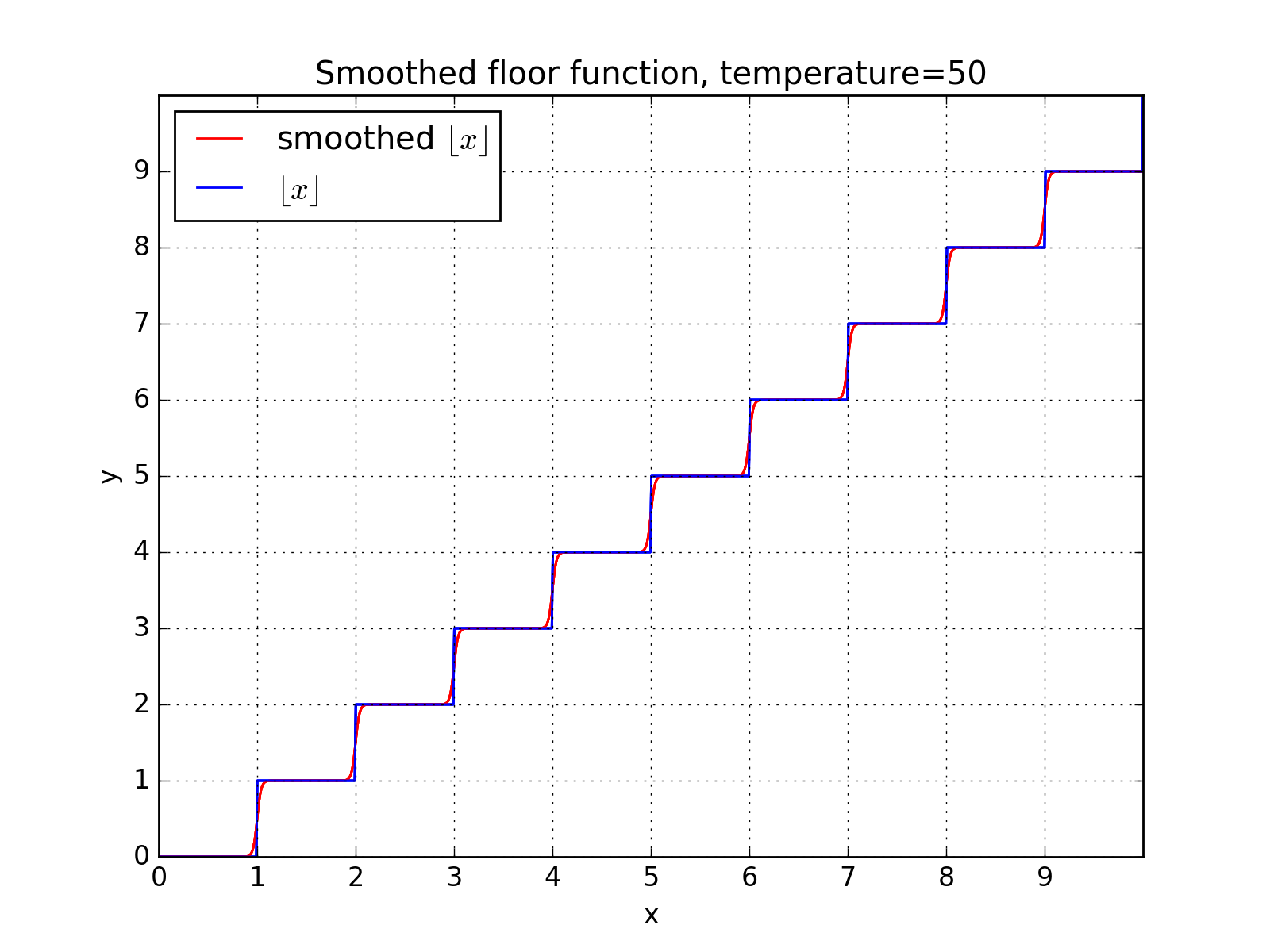
Already with a temperature parameter of 50 the smoothed function is very close to the discrete floor function.</figcaption> </figure>
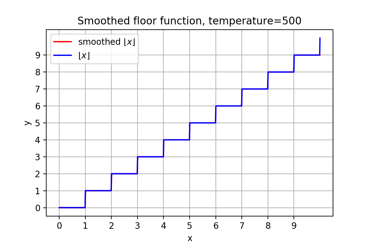
Increasing the temperature to 500 and the difference with floor cannot be noted.</figcaption> </figure>
Let's talk!
I'm Carlo Nicolini — I am interested on the reliability of AI reasoning systems (interpretability, inference-time methods, probabilistic language programming) and on quantitative portfolio optimization (I am a maintainer of skfolio). If you're working on something in these areas and think we might collaborate, chat, discuss, I'm happy to talk about it!
The best way to reach me is on via DM on LinkedIn.