This short blog note is covering some aspects related to interesting calculations that can be done in random matrix theory applied to the study of spectral properties of random graph models, like those shown in Figure:

Figure 1. Some random graph models. (a) Erdos-Renyi, (b) Gilbert model, (c) Geometric, (d) Barabasi-Albert, (e) Watts-Strogatz, (f) k-regular. Taken from Dehmer2015.
We want to study the properties of some random graph ensemble in terms of the spectral density of the eigenvalues of the Laplacian. We denote the adjacency matrix of a random graph as \(\mathbf{A}\), its Laplacian of \(\mathbf{L}\). The parameters of the random graph model are indicated by the parameters \(\boldsymbol \theta\), so we can imagine every single random graph is a collection of \(n(n-1)/2\) random variables dependent on the parameters \(\boldsymbol \theta\).
We are interested in the limiting distribution of the ensemble eigenvalues, a quantity known as the average spectral density \(\mathbb{E}[{\varrho}]\), where by the operator \(\mathbb{E}[\cdot]\) we mean the ensemble average at constant parameters \(\boldsymbol \theta\). This is also indicated in statistical physics with the triangular brackes \(\langle \cdot \rangle\).
Numerically we could in principle compute a large number of random adjacency matrices from the graph ensemble and obtain the spectral density via histogramming. However we have more powerful tools to accomplish this task: the matrix resolvent and the Stieltjes transform.
We can obviously write the spectral density \(\varrho\) of a matrix \(\mathbf{L}\) with the help of the Dirac delta function as: \(\varrho(z) = \frac{1}{n}\sum_{i=1}^n \delta(z-\lambda_i)\) where \(\lambda_i\) are the eigenvalues of the matrix.
We can invoke to the so-called Plemelij-Sokhotski formula, to write the delta function as the limit in the complex plane approaching the real line of the imaginary part of the following quantity: \(\delta(x) = -\frac{1}{\pi} \lim \limits_{\eta \to 0^+} \mathrm{Im} {\frac{1}{x + i \eta } }.\)
Hence, for the spectral density we recover the following expression: \(\varrho(x) = -\frac{1}{n \pi} \lim \limits_{\eta \to 0^+} \mathrm{Im} {\sum \limits_{i=1}^n \frac{1}{x + i \eta - \lambda_i} }.\) Now we identify the complex variable \(z=x+i \eta\) and thanks to a change of basis and the properties of matrix functions, we can evaluate the sum in the argument of the imaginary function as: \(\sum \limits_{i=1}^n \frac{1}{x + i \eta -\lambda_i } = \mathrm{Tr}{(z \mathbf{I} - \mathbf{L})^{-1}}\) The function \(R(z)=(z\mathbf{I} -\mathbf{L})^{-1}\) is called the resolvent matrix of \(\mathbf{L}\). By averaging over the resolvent we can get an expression for the expected spectral density over the ensemble of random matrices denoted by \(\mathbf{L}(\boldsymbol{\theta})\): \(\mathbb{E}[{\varrho(z)}] = -\frac{1}{n \pi} \lim \limits_{\eta \to 0^+} \mathrm{Im}{ \mathrm{Tr}{ \mathbb{E}{ (z I - \mathbf{L} )^{-1} } }}\) where the expectation is taken over the ensemble of networks \(\mathbf{L}\) with parameters \(\boldsymbol{\theta}\). The quantity \(\mathrm{Tr}{(z I - \mathbf{L} )^{-1}}/n\) is called the Stieltjes transform. Importantly the resolvent is the generating function of the moments \(\mu_k=\mathbb{E}[{\mathrm{Tr}{\mathbf{L}^k}}]\) of the spectral density: \(\mathbb{E}\left \lbrack{ (z I - \mathbf{L} )^{-1} }\right \rbrack = \int dx' \frac{\varrho(x')}{z-x'} = \frac{1}{z}\sum_{k=0}^{\infty} dx' \varrho(x') \left( \frac{x'}{z}^k \right) = \sum_{k=0}^{\infty} \frac{\mu_k}{z^{k+1}}\) where, by normalization of the density \(\mu_0=1\). In general we can compute the average traces of a random matrix \(\mathbf{X}\) by means of integrals over their spectral density: \(\mathbb{E}[{\mathrm{Tr}{[\mathbf{X}^k]}}]= n \int d\lambda \lambda^k \varrho(\lambda | \mathbf{X}).\) In the rest of this document, to simplify notation we identify the average spectral density \(\mathbb{E}\lbrack{\varrho}\rbrack\) simply as \(\varrho\). This also apply in the case of matrix functions, thanks to the series expansion. Being the expression for the moments \(\mathbb{E}[\mathrm{Tr}[\mathbf{X}^k]]\) always valid, thanks to series expansion of some generic matrix function \(f(\mathbf{X})\) we can extend this result to general functions \(f\).
If we choose the often encoutered statistical mechanical quantity \(f(\mathbf{X}):=e^{-\beta \mathbf{X}}\) we obtain this nice expression for the calculation of the expected partition function of a random graph ensemble in the spectral entropies framework: \(\mathbb{E}\left \lbrack{\mathrm{Tr}{e^{-\beta \mathbf{L}}}} \right \rbrack = n \int \limits_{0}^{\infty} e^{-\beta z} \varrho(z) dz\)
We can then compute the average spectral density as: \(\rho(x) = -\frac{1}{\pi n} \lim \limits_{\epsilon \to 0^+} \mathrm{Im} \left \langle \sum \limits_{i=1}^n \frac{1}{\lambda_i + j\epsilon - x} \right \rangle\)
If you find this example useful, feel free to contact me.
Numerical implementation
All this stuff is pretty nice, mathematically. But we like numerical calculations and want to see if all this theory applies.
So we try to numerically compute the ensemble laplacian spectral density by means of the Stieltjes transform of the Laplacian of the Erdos-Renyi random graph.
With the function LER we define sample the Laplacian of a network with n nodes and parameter p.
Here is the Python code to compute the spectral density of a random matrix ensemble via the average resolvent.
import numpy as np
from scipy.linalg import eigvalsh
import matplotlib.pyplot as plt

# Function to generate the Laplacian of a Erdos-Renyi random graph with n nodes
# and parameter p
def LER(n,p):
    X = np.random.random([n,n])
    X = (X+X.T)/2
    np.fill_diagonal(X,0)
    A = (X<=p).astype(float)
    L = np.diag(A.sum(axis=0))-A
    return L

def spectral_density_laplacian_er(n,p,x,reps,eps=1E-1):
    def resolvent_trace(x,lambdai):
        return np.sum([1.0/(xi+1j*eps-x) for xi in lambdai])
    def average_resolvent_trace(x):
        return np.mean([resolvent_trace(x, eigvalsh(LER(n,p)) ) for r in range(0,reps)])
    return [-1/(np.pi*n)*np.imag(average_resolvent_trace(z)) for z in x]
Let us put our theory at work and generate the spectral density with a chosen level of detail:
n=200
p=0.25
x=np.linspace(0,50,100)
reps=500
rho = spectral_density_laplacian_er(n,p,x,reps)
plt.plot(x,rho)
plt.hist(np.array([eigvalsh(LER(n,p)) for r in range(0,1000)]).flatten(),100,normed='freq')
plt.xlabel('$$\\lambda$$')
plt.ylabel('$$\\varrho(\\lambda)$$')
plt.title('Spectral density Erdos-Renyi Laplacian N=200 p=0.25')
plt.show()
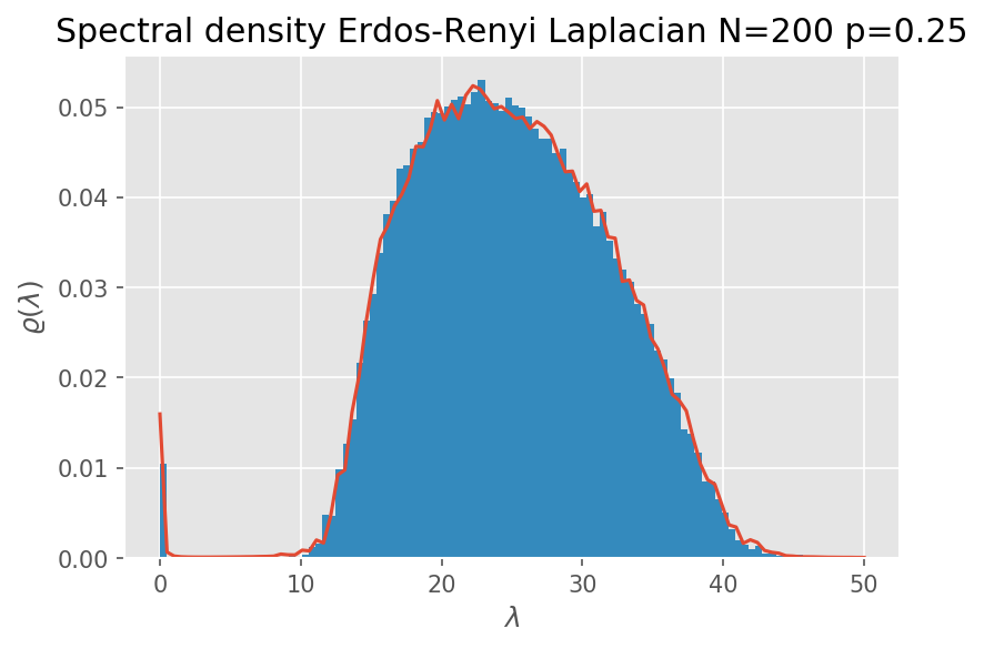
Spectral density Erdos-Renyi Laplacian N=200 p=0.25</figcaption> </figure>
The \(\epsilon\) parameter (eps in the code) is the one present in the limit.
While analytically a limit procedure should be computed, the parameter controls approximately the bin size of an histogram. A not too big value (in the order 0.1) and the noise of the expectations is averaged out.
If you increase the number of repetitions and limit the eps parameter very close to zero, being cautios to avoid underflows, you can reconstruct the exact limiting distribution as observed in the histogram.
To get a smoother curve either you analytically calculate the formula for the spectral density, or you largely increase the number of samples. At the moment there is not closed form formula for the Laplacian of the Erdos-Renyi graph. A numerical solution comes from the Peixoto paper (Eigenvalue spectra of modular networks).
References
To make this blog post I have read a few papers on random matrix theory in graph theory and complex networks. The most important reads are the following:
- Nadakuditi, Raj Rao, and Mark EJ Newman. “Graph spectra and the detectability of community structure in networks.” Physical review letters 108.18 (2012): 188701.
- Nadakuditi, R. R., & Newman, M. E. (2013). Spectra of random graphs with arbitrary expected degrees. Physical Review E, 87(1), 012803.
- Peixoto, T. P. (2013). Eigenvalue spectra of modular networks. Physical review letters, 111(9), 098701.
- Edwards, S. F., & Jones, R. C. (1976). The eigenvalue spectrum of a large symmetric random matrix. Journal of Physics A: Mathematical and General, 9(10), 1595.
- Livan, G., Novaes, M., & Vivo, P. (2018). Introduction to Random Matrices: Theory and Practice. Springer International Publishing.
- Dehmer, M., Emmert-streib, F., Chen, Z., Li, X., Barabási, A., n.d. Mathematical Foundations and Applications of Graph Entropy ``Quantitative and Network Biology’’.
Let's talk!
I'm Carlo Nicolini — I am interested on the reliability of AI reasoning systems (interpretability, inference-time methods, probabilistic language programming) and on quantitative portfolio optimization (I am a maintainer of skfolio). If you're working on something in these areas and think we might collaborate, chat, discuss, I'm happy to talk about it!
The best way to reach me is on via DM on LinkedIn.