Comparing spectral densities of random graph models.

The ability of quantitatively comparing two graphs is of great importance in many scientific questions and of exceptional importance in studying brain networks. How the brain networks of healthy people differ from those of patients? What kind of alterations are present in the functional connectivity of diseased brain? To what extent two networks are structurally similar?

To answer these questions, many graph measures have been developed, but no approach starts from ground principles. Information theory and statistics are two disciplines that must bring their ideas into complex networks science. In particular an idea that is emerging is that different graphs must differ in their spectra, i.e. the distribution of their eigenvalues. It turned out indeed, that the empirical distribution of the eigenvalues of adjacency matrices of graphs, can tell us more about the general properties of the network than some other aggregate measures, like for example the degree distribution, or other metrics.

Additionally, a deep parallel connection seems to exist between complex networks and quantum physics and recently this connection is under investigation by researchers in complex networks, mathematics and physics. The ideas of the physics of information, and in particular the concept of entropy both in the physical and information theoretic views, is of great importance also when applied to complex networks.

Apart from this details, here we expose the most basic ideas in the field, always keeping in mind that our final target is to find a way to compare graphs (and subgraphs) in a theoretical sound manner. To do this, let’s start from the most basic concepts in graph theory, by introducing the mathematical notation.

Notation

A graph \(G =(V,E)\) is an ordered pair, where \(V =\{1, 2,\ldots, n\}\) is a set of vertices and \(E\) is a set of edges connecting the elements of \(V\). All graphs considered in this notes are undirected, that is, each edge \(e \in E\) is an unordered pair of vertices. The spectrum of \(G\) is the set of eigenvalues of its adjacency matrix, which is denoted by \(\mathbf{A}\). Two vertices \(i\) and \(j\) are connected by an edge, if \(A_{G_{ij}} = 1\), otherwise, \(A_{G_{ij}}=0\). In undirected graphs, we have \(\mathbf{A} = \mathbf{A}^T\), therefore, all eigenvalues of the matrix \(A_G\) are real.

Random graph models

Random graph models are probabilistic generative models that, given a set of parameters, yield different instances of random graphs. Among the most famous examples of random graph models we can list:

• Erdos-Renyi model, also called \(G(n,m)\) model, where \(n\) nodes and exactly \(m\) edges are connected randomly. Here the number of edges is fixed (microcanonical description).
• Gilbert model, also called \(G(n,p)\) model, where \(n\) nodes are connected randomly with probability \(0 \leq p \leq 1\)). Here the number of edges is on average \(\left <m \right >=p n(n-1)/2\) (canonical description).
• Watts-Strogatz model, a model that generates networks with scale-free degree distribution.
• Barabasi-Albert model, also called preferential attachment model.
• Random regular graph model, where every node has exactly degree \(k\).
• Planted partition model, a block model where the intra-block density \(p_{in}\) and extra-block density \(p_{out}\) are parameters.

In more formal terms, a random graph model is an algorithm that describes the construction of a random graph given a probability space \((\Omega,\mathcal{F},P)\), where the sample space \(\Omega\) is a nonempty set of graphs, the set of events \(\mathcal{F}\) is a collection of subsets of the sample space (usually is the power set of \(\Omega\)), and \(P\) is a function that assigns a probability to each event.

Is it possible then, given a random graph \(G\) to infer which random graph model it belongs? This problem is partially related to the inference problem in statistics and uses tools from information theory. Finding an appropriate answer to this question can solve the problem of graph comparison, namely, given two graphs \(G_1\) and \(G_2\) to what level of confidence can we measure their structural similarity and infer whether they are from the same random graph model?

Figure 1: Some random graph models. (a) Erdos-Renyi, (b) Gilbert model, (c) Geometric, (d) Barabasi-Albert, (e) Watts-Strogatz, (f) k-regular. Taken from Dehmer2015.

Spectral density

The eigenvalue decomposition of the adjacency matrix \(\mathbf{A}\) (a real symmetric \(n\times n\) matrix) is the following:

where \(\mathbf{Q}\) is the eigenvectors matrix and \(\mathbf{\Lambda}\) is the eigenvalues diagonal matrix. One can then take the diagonal elements of the matrix \(\mathbf{\Lambda}\), i.e. the set \(\{\lambda_1, \ldots \lambda_n\}\) and get its empirical distribution, that here we indicate with \(\mathbf{\rho}\).

The spectral graph theory studies graph spectra properties and their association with the graph structure. It is easy to get convinced that the graph eigenvalues contain much information about the graph, indeed here I show just some nice properties of the graph eigenvalues.

1. Let \(k_i\) denote the degree of \(i\). Then the eigenvalue \(\lambda_1\) is at least \(\frac{1}{n}\sum_{i=1}^n k_i\).
2. The graph \(G\) is bipartite if and only if \(\lambda_n = -\lambda_1\) (in general bipartite graphs have symmetric spectrum)
3. If \(G\) is connected, then the eigenvalue \(\lambda_1\) is strictly larger than \(\lambda_2\) and there exist a positive eigenvector of \(\lambda_1\). The largest eigenvalue \(\lambda_1\) is also called the Perron-Frobenius eigenvalue.
4. Each vertex in \(V\) is connected to exactly \(\lambda_1\) vertices only if the vector of ones is an eigenvector of \(\lambda_1\).
5. Let \(C \subset V\) such that each pair of vertices in \(C\) are connected in \(G\), i.e. \(C\) is a clique in \(G\). Then, the size of \(C\) is at most \(\lambda_1 + 1\).
6. Let \(d\) be the diameter of \(G\). If \(G\) is connected, then \(A_G\) has at least \(d+1\) distinct eigenvalues.

From spectrum of a single graph to the spectrum of a graph model

More interesting than the eigenvalues spectrum of a single graph is the spectral density of eigenvalues of a family of graphs. For families of graphs, a colloquial term to indicate a random graph model, indeed, one can compute the spectral distribution of eigenvalues, dubbed its spectral density.

The definition of spectral density is based upon the definition of a limit. In the case where analytical estimates are not possible, the estimate of spectral density is based on the computation of eigenvalues of a large number of graphs. Precisely, if \(\lambda_i(G)\) are the eigenvalues of a single graph, then the empirical spectral density of \(G\) is defined as

where \(\lambda\) is the continuous distribution of eigenvalues that is estimated by discrete \(\lambda_i\). In the limit of large networks then, the spectral density of a certain random graph model is computed as:

I will give more operational definitions of these two formulas in the next sections.

In Figure 2 the spectral densities for two families of graphs are displayed. On the left, the spectral density for a Erdos-Renyi model with \(N=500\) nodes and connection density \(p=0.05\). On the right, the same for a Gilbert model with \(N=500\) nodes and \(20\) edges. As the density \(p<0.5\) then more than one connected component exist, generating then many zeros in the eigenvalue spectrum.

Figure 1: Spectral densities estimated for Erdos-Renyi and Gilbert random graph models (left and right respectively).

Interestingly, the spectral density of k-regular graphs is analytically calculable and can be written in the following form:

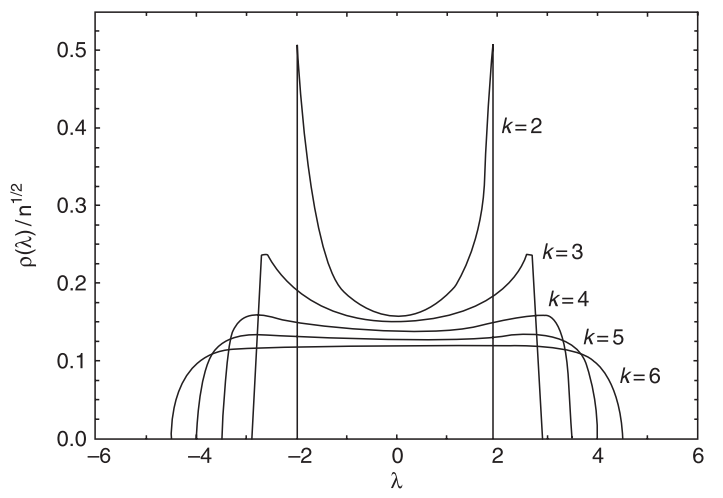
Figure 3: Spectral density of a k-regular network. Taken from Estrada 2013

Studying the spectral density of random graph models is a rather powerful tool to identify different graph models, as they act as some “fingerprint” of the stochastic process that generates them.

Spectral entropy

Any random graph model is characterized by a spectral density, a continuos probability function that describes the relative frequency of its eigenvalues, given some parameters. In trying to establish a “network information theory”, it appears that the spectral density is important to define the so-called graph spectral entropy.

Different forms of entropies of graphs have been defined , and typically they rely on some application of classical Shannon entropy to some probability distributions obtained for graphs. The spectral entropy \(S(G)\) of a random graph model is defined in terms of continuos probability distributions as:

Operatively, to approximate the entropy of a random graph, one may use the random graph model to construct many graphs, and then estimate the spectral density from that data set. For example, given a random graph model, we construct a set of graphs \(\{G_1,G_2,\ldots,G_N\}\) with \(n\) vertices using the model, and then for each \(G_j,1 \leq j \leq N\), we apply a density function estimator.

In the examples shown here, we consider an estimator based on the Gaussian kernel. It can be interpreted as a smoothed version of a histogram. Given a graph \(G_j\) and its spectrum \(\{\lambda_1^{(j)}, \ldots, \lambda_n^{(j)} \}\) each eigenvalue \(\lambda_i\) contributes to estimate the function in a point \(\lambda\) according to the difference between \(\lambda_i\) and \(\lambda\). That contribution is weighted by the kernel \((K)\) function and depends on a parameter known as bandwidth \((h)\), which controls the size of the neighborhood around \(\lambda\). Formally, the density function estimator in a point \(\lambda\) is:

where \(K(u)=(\sqrt{2 \pi})^{-1} \exp(-u^2/2)\).

In the case where analytical calculations are possible as in the ER model with link probability \(p\), the spectral entropy can be computed analytically as:

then, the maximum spectral entropy of the ER random graph is achieved when \(p = 0.50\).

This is consistent with the intuitive idea that when all possible outcomes have the same probability to occur, the ability to predict the system is poor. By contrast when \(p \rightarrow 0\) or \(p \rightarrow 1\), the construction of the graph becomes deterministic and the amount of uncertainty associated with the graph structure achieves its minimum.

In a 2012 paper, Takahashi introduced comparison of spectral densities of graph models as the tool for the identification of differences between groups of brain networks. Additionally, they proposed general methods for model selection and network model parameter estimation, as well as a statistical procedure to test the nullity of divergence between two classes of complex networks.

Model selection in graphs?

To learn statistical methods in graphs, we must first understand the concept of probability distribution over graphs. The theory behind it is the theory of random graphs, which studies the intersection between graph theory and probability theory. As example, a random graph model is the Erdos-Renyi, in which the sample space \(\Omega\) is the set of all graphs having \(n\) labeled vertices, and \(m\) edges (usually \(m\) is a function of \(n\)). Each graph of \(\Omega\) can be generated by selecting \(m\) edges from the \(\binom{n}{2}\) possible edges. Therefore, the set \(\Omega\) has size \(\binom{\binom{n}{2}}{m}\) and the probability to choose a graph from \(\Omega\) is given by:

\(\Pr = \left( \binom{\binom{n}{2}}{m} \right)^{-1}\).

Suppose now that we take at random two graphs \(G_1\) and \(G_2\), each one of size \(n\). If both graphs are from the same random graph model, then it is reasonable to expect that in the limit \(n \rightarrow \infty\) they share some structural properties. By contrast if \(G_1\) and \(G_2\) are from different graph models, we may expect to find fundamental differences between their structural properties.

Given the graphs \(G_1\) and \(G_2\), can we measure the similarities between their structures? Is the probability of \(G_1\) and \(G_2\) being from the same random graph high? To answer these questions, we need a mathematical way to describe graph structural properties that are equal for graphs from the same random graph, but different for elements from distinct random graphs.

Takahashi proposed that the spectrum of a graph is an adequate summarization of the graph structure for this problem. In the following section, we define the graph spectrum and other spectrum-based concepts that describe a set of graph structural properties.

Kullback-Leibler divergence

As the entropy of random graphs is defined, it comes natural to implement some sort of measure of graph distance in terms of spectal densities, i.e. to start doing information theory on networks.

Practical implementation and code

In the following pieces of code, we try to compute the spectral densities of the Erdos-Renyi Gnp random graph model, using Python libraries as numpy,networkx and matplotlib. In the case you don’t have those libraries, I suggest to look for them with pip or simply easy_install.

To estimate the continuous distribution of the spectral densities we rely on a Montecarlo-like simulation. The idea is to generate many instances from the specific random graph model and on each instance compute the eigenvalues.

We then average the eigenvalues and compute the continuous density function with the help of a kernel density estimator. As density estimatore we use Gaussian Kernels where the bandwidth of the kernel is found by the Silverman criterion as in the original work upon which this article is based.

We now import all the Python libraries useful for this task:

"""
See the book Mathias Dehmer,
"Mathematical Foundations and Applications of Graph Entropy"
Chapter 6 Statistical Methods in Graphs: Parameter Estimation, Model Selection, and Hypothesis Test
"""
import networkx as nx
import numpy as np
import matplotlib.pyplot as plt
import seaborn as sbn
from numpy.linalg import eigvals
from scipy import stats

Then we focus on the estimation of the spectral density of the ER model \(G(n,p)\) that in some sense is the canonical ensemble version of the \(G(n,m)\) random graph model (the microcanonical ensemble where number of links is an hard constraint). We use a \(p=0.007\) and generate 1000 random graphs of \(n=50\) nodes, computing then the average eigenvalues.

# Generate 1000 ER random graphs with the Erdos-Renyi model 
# and compute their eigenvalues mean
n = 50
p = 0.05
nsamples = 10000
vs = np.array([0]*n)
for i in range(0,nsamples):
    G = nx.gnp_random_graph(n,p)
    A = nx.to_numpy_matrix(G)
    v = np.real(eigvals(A))
    vs = vs + v
vs = vs/nsamples

We must divide the average eigenvalue by \(\sqrt(n)\) and then estimate the Gaussian Kernel Density.

vs = vs/(np.sqrt(n))
kde = stats.gaussian_kde(vs,bw_method='silverman')
x = np.linspace(vs.min(), vs.max(), 100)
rho = kde(x)

Finally we plot the empirical data together with the theoretical analytical estimate:

plt.plot(x,rho)
plt.ylabel('Spectral density')
plt.xlabel('Eigenvalues')
plt.title('ER Model spectral density')

with the following (nice) result about the ER spectral density:

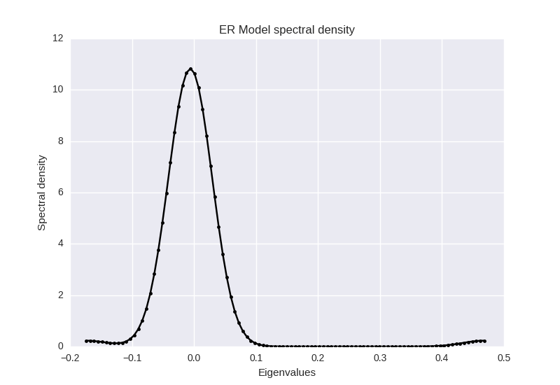
Figure 3: Spectral densities computed for Erdos-Renyi graph. \(N=50, p=0.05\).

References

• Dehmer, M., Emmert-streib, F., Chen, Z., Li, X., Barabási, A., n.d. Mathematical Foundations and Applications of Graph Entropy “ Quantitative and Network Biology ” Advisory Board : Previous Volumes of this Series : Applied Statistics for Network Advances in Network Statistical Modelling of QSAR / QSPR Statistical Diagnost.

• Takahashi, D.Y., Sato, J.R., Ferreira, C.E., Fujita, A., 2012. “Discriminating Different Classes of Biological Networks by Analyzing the Graphs Spectra Distribution”. PLoS One 7. doi:10.1371/journal.pone.0049949

• Estrada, E., 2013. The structure of complex networks. doi:10.1017/CBO9781107415324.004